Installing and starting up R
This page contains step-by-step instructions for installing and running R and R Studio. It will also introduce you to some concepts when talking to R. It is highly recommended that you complete the swirl course R programming
Learning objectives
By the end of this session you will be able to answer these questions:
- What is R and RStudio?
- How can I interact with R?
- What are the components of RStudio
- What is a reproducible computing?
- How do I maintain a reproducible work-flow in R and RStudio?
Installing R
R is a free, open-source software designed for statistical computing. To download and install R:
- Go to https://cran.uib.no/,
- select your operating system (Download R for Windows, MacOS or Linux).
- If you have Windows, choose
base, click on “Download R (…) for windows”, save and run the file. The installation process should be self explanatory. - If you have MacOS, download and install the latest release.
- If you have Windows, choose
Installing R Studio
RStudio is a software designed to make it easier to use R. Install it by going to https://www.rstudio.com/. It is free to download and use.
- Select “Products” and RStudio
- Go to desktop and select “DOWNLOAD RSTUDIO DESKTOP”
- Select the free open source license and download the file made for your operating system (use the installers).
Getting to know R and RStudio
R is a software used for scientific/statistical computing. If R is the engine, RStudio is the rest of the car. What does this mean?
When doing operations in R, you are actually interacting with R through RStudio. RStudio have some important components to help you interact with R.
The source
The source is where you keep your code. When writing your code in a text-file, you can call it a script, this is essentially a computer program where you tell R what to do. It is executed from top to bottom. You can send one line of code, multiple lines or whole sections into R. In the image below, the source window is in the top left corner.
Environment
The environment is where all your objects are located. Objects can be variables or data sets that you are working with. In RStudio the environment is listed under the environment tab (bottom left in the image).
Copy and run the code below.
a <- c(1, 2, 4)What happened in your environment?
The console
Here you can directly interact with R. This is also where output from R is printed. In the image below, the console is in the top right corner.
Files, plots, packages and help files
In RStudio files are accessible from the Files tab. When opening a project, the files tab shows the files in you root folder.
Plots are displayed in the Plot tab. Packages are listed in the packages tab.
If you access the help files, these will be displayed in the help tab.
In the image below all these tabs are in the bottom right corner.
RStudio.
Customizing the apperance of RStudio
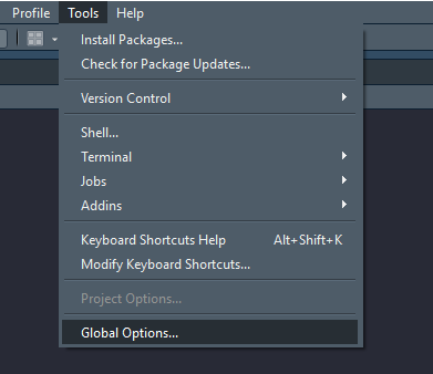
To access options for RStudio, go to Tools -> Global options
RStudio.
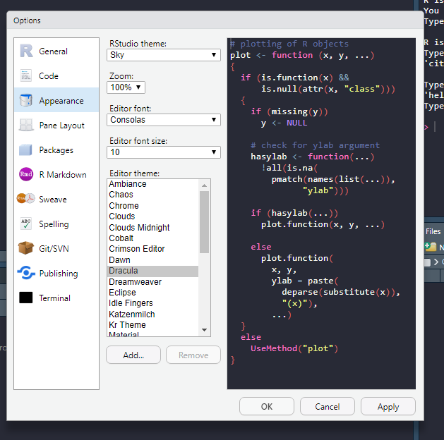
Under apperance you can customize the theme of RStudio, select something that is easy on the eye!
RStudio.
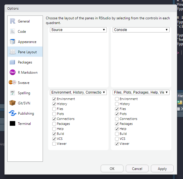
Under pane layout, you can set where you want your tabs, I like to have the source on the left, above the environment. This way you can have the source window at full vertical size and still look at plots and the console to the right.
RStudio.
Reproducible computing
Computations are reproducible when you can show how they were performed. This is achieved by creating “programs” from where your analyses are done. In R, these programs are lines or R code stored in a text-file, either .R-files or .Rmd-files. .R-files are scripts only containing code and comments. A .Rmd-file is a special script combining text and computer code, when the Rmd-file is executed, it creates a report and outputs the results from the code.
This means that to work in a reproducible way, you need to script all your operations.
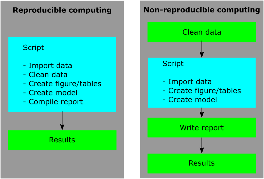
Reproducible vs. non-reproducible workflow
Importantly, in RStudio you can shut down storing temporary objects in a environment that is relaunched on start up. What is the consequence of having such a situation?
To disable this option, set save works pace to NEVER!
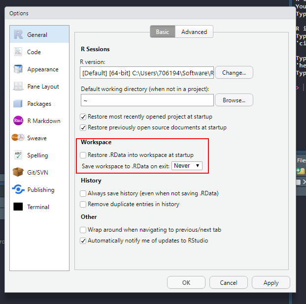
RStudio.
Start coding!
The online book Learning statistics with R has an updated chapter about installing and setting up R (Chapter 3). This chapter also goes through how commands are typed into R.
When you have installed your copy of R and RStudio, start up RStudio and type the following in the console window:
x <- 2

z <- 4

x + z
These “commands” tells R to store the number 2 in an object that we name x. Then we store the number 4 in an object named z . Next we tell R to add these two together. If you enter each command followed by pressing enter in the console, R will return the sum of x and z which should be 6.
The operations that you did above using the <- operator is called variable assignment. Read more about it in section 3.4 of Learning statistics with R.
Before going any further it can be useful to know that you can save your code as R scripts. In RStudio, go to File > New File > R Script. The R script is a text-file where you can write code that can be sent to the console. To execute a line of code, have the cursor on the line you would like to run and press Ctrl + Enter on your keyboard. If you would want to run the whole script, either press Source in the top right corner of the Source window in RStudio or select all lines and pre Ctrl + Enter. R scripts can be saved, this makes for an opportunity to make reproducible analyses. We will talk more about this later.
In the R script we can “comment out” lines of text using the # symbol. An R script with comments can look like this:
# This line is a comment, the line below is code

x <- 34

# This line is a comment, in this script only x <- 34 will be evaluated.
Types of data in R
R can store many types of data.
Scalars
Scalars are objects that can take only one value at a time. We have already worked with scalars when we assigned a single number to the objects we named x and z above. Scalars can also be TRUE or FALSE, these “are reserved words denoting logical constants in the R language”1 meaning that they have special meaning and cannot be used for assigning different values to. If we try, R returns an error message:
# Trying to assign a value to TRUE
TRUE <- 3
## Error in TRUE <- 3 : invalid (do_set) left-hand side to assignmentThe message says that the left-hand side of the assignment is invalid. TRUE is on the left-hand sign of the <- operator.
Scalars can also be character strings, this means text. We can thus store text in an object like this:
# Store text in an object, named text
text <- "This is text, more specifically a character string"
When asking R to return (or print) what is stored in the object text we will ge this in the console:
text## [1] "This is text, more specifically a character string"Vectors
A vector is an object containing multiple entries of data, or multiple scalars. These can be of different types; numeric, character or logical. A vector can be created by storing data in an object using the c()function. The c() function combines data into a vector.
numeric_vector <- c(1, 4, 6, 8) # A numeric vector
logical_vector <- c(TRUE, FALSE, TRUE, TRUE) # A logical vector
character_vector <- c("a", "character", "vector", "!")
We can access specific parts of the vector by specifying the place in the vector. For example if we want to print the word “character” from the object character_vector we access it by character_vector[2]
# Access the second element of the vector
character_vector[2]
## [1] "character"We can name the elements of the vector and access them by calling their names
# Check the names (Should be NULL, nothing there)
names(character_vector)
## NULL# Name the elements using another vector
names(character_vector) <- c("the first name", "the second name", "the third name", "the fourth name")
# Access the second element
character_vector["the second name"]## the second name
## "character"This is sometimes usefull, but more importantly, it shows how you can acces data from a vector.
One of the nice things about the R language is the mathematical operations can be done on vectors. If we multiply the numeric vector with 2, all element of the vector will be multiplied with 2.
numeric_vector * 2This command does the following:
| vector | operator | value |
|---|---|---|
| 1 | * | 2 |
| 4 | * | 2 |
| 6 | * | 2 |
| 8 | * | 2 |
If the numeric vector is multiplied with another vector of the same length, the operation is done row-wise.
numeric_vector * c(2, 1, 2, 3)| vector 1 | operator | vector 2 |
|---|---|---|
| 1 | * | 2 |
| 4 | * | 1 |
| 6 | * | 2 |
| 8 | * | 3 |
Note that if vectors are not the same length (or a multiple of shorter object length), R will give you a warning.
numeric_vector * c(2, 1, 4)## Warning in numeric_vector * c(2, 1, 4): longer object length is not a multiple of shorter object length## [1] 2 4 24 16A vector of length 4 can be multiplied with a vector length 2 as the shorter vector can be used two times over the longer vector.
Character vector can not be used in mathematical operations, try it out, what do the error message say? What does it mean?
Logical vectors can be “coerced” to numeric vector. But why do we get the results below, how do R interet the logical vector?
numeric_vector * logical_vector## [1] 1 0 6 8Data frames
We will work a lot with data frames. These are tables of data with rows and columns. A data frame can be created using the data.frame()
# Create my data frame
my_df <- data.frame(Variable1 = c(1,2,3,4), Variable2 = c(5, 5, 5, 5), Variable3 = c("one", "two", "three", "four"))
The data frame can combine different types of data into one table. The data frame can be viewed in the console by calling it, we can also access different rows and columns by specifying it when calling it e.g. using the logic my_df[row, column]
# The whole data frame
my_df
## Variable1 Variable2 Variable3
## 1 1 5 one
## 2 2 5 two
## 3 3 5 three
## 4 4 5 four# The last row
my_df[4, ]## Variable1 Variable2 Variable3
## 4 4 5 four# The firts column
my_df[,1]## [1] 1 2 3 4# The first row, second column
my_df[1,2]## [1] 5We can also access and create new columns in a data frame by using the $ operator. We can use variables in the data frame to create these new variables.
my_df$Variable4 <- my_df$Variable1 + my_df$Variable2

my_df
## Variable1 Variable2 Variable3 Variable4
## 1 1 5 one 6
## 2 2 5 two 7
## 3 3 5 three 8
## 4 4 5 four 9Later we will learn different ways of manipulating data frames that will turn out to be a bit more convinient.
Data matrices
A matrix is a type of table, similar to a data frame, but all element must be of the same type e.g. numeric.
A matrix can be created using several vectors of the same size and content. The cbind() function is used below to bind columns of numbers together.
my_matrix <- cbind(c(1,2,3,4),
                   c(4,6,8,9),
                   c(8,3,2,1))
Lists
Lists are objects containing other objects. We can combine objects in a list, this is sometimes useful for storage of data. We can name the objects in the list when listing them or by using the names() function. This is nice, because we can access it by using the $ operator.
# Store objects in a list
my_list <- list(my.vector = numeric_vector,
             my.dataframe = my_df)


my_list$my.vector
## [1] 1 4 6 8Functions
R can store data and functions. Functions are usually used to take some input, do something and return an output. R contains a lot of functions as this is the basis of how we work with data. There is no need to write functions, these are already written by others and can be used by you to analyze data or make figures. However, it can be useful to know how a function works.
A quick look! We will create a function that calculates the mean of a vector. This function already exists, it is called by the mean() command.
We can use our numeric vector and calculate its mean
mean(numeric_vector)## [1] 4.75Lets create a function that does the same:
# Define a name of the function and start the code block creating the function
# Inside function(), the arguments of the function is defined
my_mean <- function(data = data){  # The curly brackts tells R that this code is written over multiple lines (group statement)

        n <- length(data) # Length is a function that gives the number of entries in a vector

        sum <- sum(data) # Sum calculates the sum of a vector

        my_mean <- sum/n # Sum over number of entries

        return(my_mean) # return is a function (used in functions) that tells R to print a specified value

        }

# See if it works
my_mean(numeric_vector)
## [1] 4.75Our own function returns the same number as the built in function. Great success!
All functions (included or self-made) are used in the same form as for example mean(), inside parentheses you write your arguments these can be data or “settings” for the function. You will be familiar with this way of working with functions.
Packages
Functions are created with a specialized task. Functions are collected in packages made to do a series of tasks, usually within a specific area. In this course we will use different packages, for example dplyr, tidyr and ggplot2. These have to be installed through R/RStudio.
To install a package, you use the install.packages() function. You only need to do this once.
install.packages("dplyr")To use a package, you have to load it into your environment. Use the library() function to load a package.
library("dplyr")Looking for help
In this course you will trained to do and communicate analyses of data. Often, an analysis require that you do stuff that you have never done before with software you have never used. This means that you need to develope your problem-solving skills. A good thing about using the R ecosystem is that there is a lot of help online. The key is to know what to look for!
When you google a more general concept, like “importing data into R”, there are alot of websites with guides on how to do that. For example Quick-R has really good step-by-step instructions.
When you google a specific problem like “how do i interpret results from lm in r”, you will usually find results from StackExchange/Cross validate (for example this). These are forum posts answered by very knowledge people. Often multiple answers are given to forum questions, the best answer gets more attention so it is easy to find.
There are many blogposts, websites and other resources that describe specific analyses. Learn how to read them and you will increase your chances of solving your analysis tasks.
Inside R, you always have the R documentation. If you are interested in a specific function, for example lm(), type ?lm in your console and you will access the help files.
Resources
The above is not at all a complete introduction to data types, functions or usage. Below are some useful resources to have at hand when you discover R:
- Quick R contains several tutorials, including Data types and creating new variables.
- Learning statistics with R Chapter 3 is a good introduction to R.
This is information from the R documentation, these can be accessed using the
?symbol followed by a name of a function, e.g.?logicaltyped into the console↩︎