Feedback 3: Regression models
Comparing regression to an ordinary t-test
Remember that the t-test compares two means (or a single mean against a hypothetical or known average). Comparisons can be made within the same participants or between unrelated participants. The t-test is limited to comparing two averages. The regression model is more flexible, we may compare unrelated observations (two groups) against each other using a dummy variable and this would be equivalent to a t-test.
The main aim of this first assignment was for you to see this connection.
Using the Haun data set we can see that the t-test is performed also in the regression model.
library(tidyverse)

haun <- read_csv("./data/hypertrophy.csv") %>%
  select(SUB_ID, CLUSTER, AVG_CSA_T1) %>%
  drop_na(CLUSTER)

t_results <- t.test(AVG_CSA_T1 ~ CLUSTER, data = haun, var.equal = TRUE)

reg_model <- lm(AVG_CSA_T1 ~ CLUSTER, data = haun)| Mean difference | Mean of group 1 | Mean of group 2 | t-value | p-value |
|---|---|---|---|---|
| -950 | 3588 | 4539 | -2.749 | 0.013 |
| Term | Estimate | SE | t-value | p-value |
|---|---|---|---|---|
| (Intercept) | 3588 | 244 | 14.683 | 0.000 |
| CLUSTERLOW | 950 | 346 | 2.749 | 0.013 |
In Table 1 and 2 we can see that the t- and p- values are identical for the test of differences between groups. The Regression model (Table 2) does the exact same test as the t-test (a t-test). The minus sign in the estimate and t-value of the t-test is due to different orders of the cluster variable in the different tests.
The highlighted row in Table 2 shows the coefficients associated with the LOW cluster. We can read this as the difference between the intercept in the model (which is the mean of the HIGH group) and the LOW group. This is the same comparison that is performed in the t-test.
Associations between variables
Many of you used a correlation to determine the relationship between variables in the data set. A correlation analysis contains the same information as is contained within a regression model with the same two variables. Similar to the difference between regression and t-tests, the correlation is limited to to variables whereas the regression is flexible and may be extended.
There are several variables in the data set that could be interpreted as surrogate measures of muscle mass. In the code below, these variables are selected.
haun <- read_csv("./data/hypertrophy.csv") %>%
  select(SUB_ID,
         Squat_3RM_kg, # The 3RM squat variable (strength)
         DXA_LBM_1,  # Lean body mass at time 1 (kg), not all muscle but most of it!
         AVG_CSA_T1, # Average cross sectional area irrespective of fiber type
         FAST_CSA_T1, # Average CSA of fast
         SLOW_CSA_T1) # and slow fibers
All variables can be plotted together using the plot function.
plot(haun[, -1]) # -1 for removing the SUB_ID variable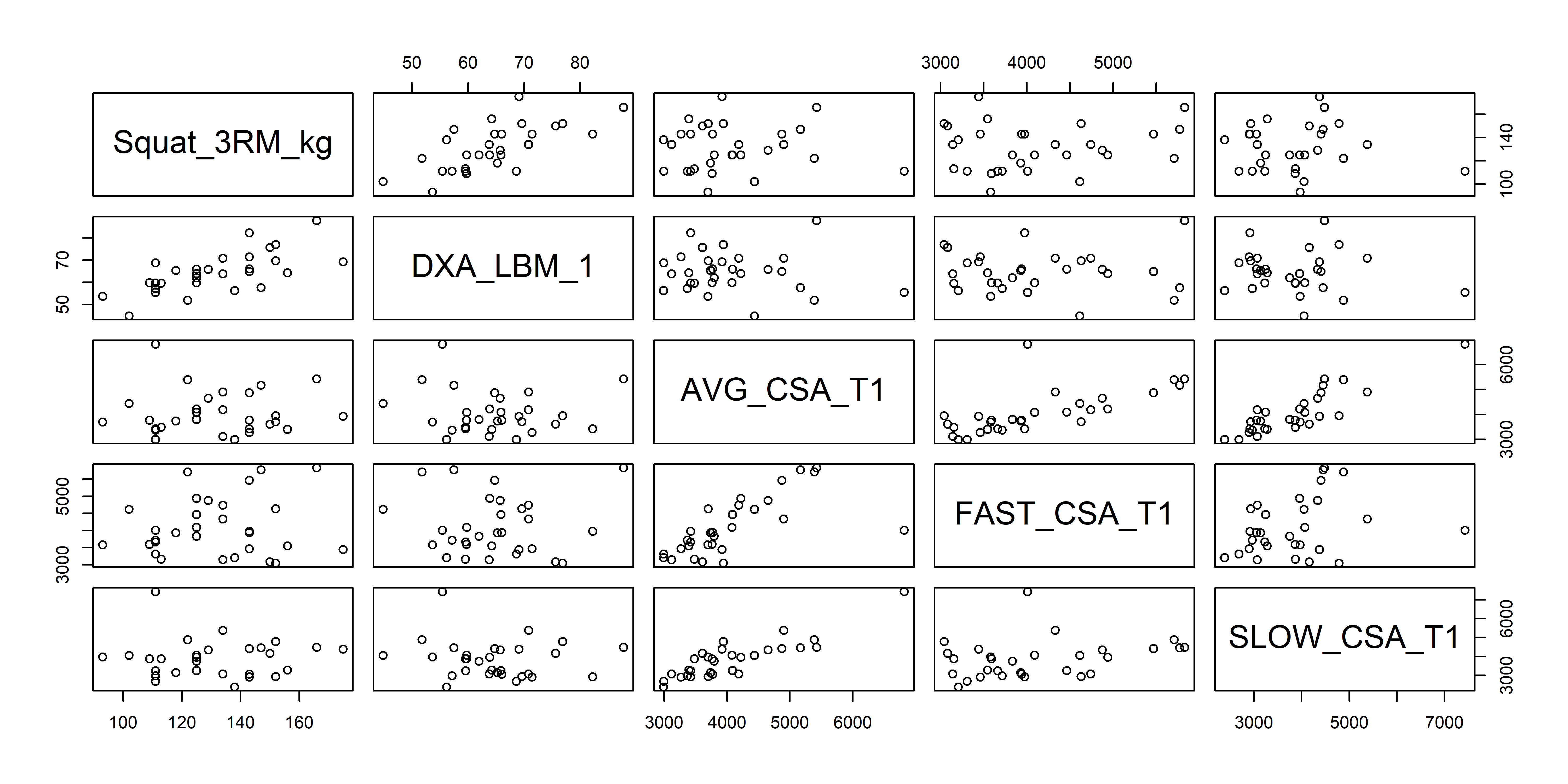
Figure 1. Interrelation between variables in selected strength and muscle-mass variables.
The plot (Figure 1) can be read as pairwise associations between variables. There seems to be a stronger association between Squat_3RM_kg and DXA_LBM_1 than between Squat_3RM_kg and AVG_CSA_T1. To assess this we can choose to do regression or correlation analysis.
A correlation analysis will give us a unit less number between -1 and 1 where number close to 0 indicates no or low association and numbers close to -1 or 1 indicates association. To assess the association between these variables using a correlation analysis
| Variables | Estimates (r) | Statistic (t) | p-value | Lower CI | Upper CI |
|---|---|---|---|---|---|
| Squat 3RM and DXA | 0.674 | 4.829 | 0.000044 | 0.415 | 0.832 |
| Squat 3RM and average CSA | 0.021 | 0.109 | 0.913598 | -0.342 | 0.378 |
As evident from Table 3, the association between 3RM Squat and lean body mass is stronger than the association between 3RM and average CSA. We see that there is a significant association between lean body mass and 3RM squat.
A regression analysis contains the same information as the correlation when we use the same variables.
# Fitting the regression model
model <- lm(Squat_3RM_kg ~  DXA_LBM_1, data = haun)
# Setting up the correlation analysis
cor <- cor.test(haun$Squat_3RM_kg,  haun$DXA_LBM_1)
In Table 4 results from the regression model are displayed. In addition to the coefficients from the regression model, I have added the R-squared (R2) value. This is actually the same as the correlation coefficient squared from the correlation analysis (In table 3). Comparing Table 3 and 4 we see that the p-values are the same when looking at the DXA_LBM_1 coefficient.
| Term | Estimate | SE | t-value | p-value |
|---|---|---|---|---|
| (Intercept) | 37.05 | 19.705 | 1.88 | 0.070534 |
| DXA_LBM_1 | 1.46 | 0.302 | 4.83 | 0.000044 |
| R2 | 0.45 | NA | NA | NA |
The interpretation of the regression table is that the average 3RM squat (kg) is 37 when we set DXA_LBM_1 to zero. Remember that the interpretation of the intercept is the value of the dependent variable (y) when all x-values are set to 0. For each unit increase in lean body mass (DXA_LBM_1) 3RM squat is predicted to increase with 1.46 kg. This effect is significant (evident from the p-value, the null hypothesis has little support).
The nice thing about the regression is that we can extend it by adding more variables to the model. Let’s say that we want to see if muscle fiber cross sectional area is more strongly associated with squat 3RM when we control for lean body mass.
# Fit the model
model <- lm(Squat_3RM_kg ~  DXA_LBM_1 + AVG_CSA_T1, data = haun)
# Check the model
summary(model)| Term | Estimate | SE | t-value | p-value |
|---|---|---|---|---|
| (Intercept) | 27.52 | 25.022 | 1.10 | 0.281060 |
| DXA_LBM_1 | 1.48 | 0.307 | 4.82 | 0.000050 |
| AVG_CSA_T1 | 0.00 | 0.003 | 0.63 | 0.534587 |
| R2 | 0.46 | NA | NA | NA |
The amount of variation that the model explained did not increase compared to the model in Table 4 as the R2 value did not increase. We can say that the about 46% of the variation in 3RM squat is explained by the two variables. As we did not see an increase in R2 we will not see a strong association between AVG_CSA_T1 and 3RM squat either. And indeed, the effect is negligible, for each unit of increase in AVG_CSA_T1 3RM does not change. The p-value indicates that the null hypothesis cannot be rejected with any confidence.
Intepretation
Many of you have interpreted the model but not the meaning of it. Based on the models in Table 4 and 5 we may say that lean body mass is positively related to strength. If we measure more lean body mass, we will likely have a stronger individual compared to an individual with lower lean body mass. The average cross sectional area does not however predict strength.
Lactate thresholds and regression analysis
The last part of the assignment was an example of regression analysis and prediction. In the physiology lab you collected lactate values. A simple regression model can be used to accurately predict workload at a fixed lactate value. Some of you will most likely use models like these in your master thesis.