Pre- to post-treatment analysis

1 Background

In sport science (and e.g. medical-, nutritional-, psychological-sciences), intervention-studies are common. We are interested in the effect of e.g. a training method, nutritional supplement or drug. The outcome in these studies could be physical performance, degree of symptoms, muscle size or some other measure that we are interested in studying. These studies are often called Randomized Controlled Trials (RCT)

The choice of study design relates to the research-question and dictates what statistical methods can be applied. The study design affects the ability of the study to detect an effect (the power). A common case of a RCT is the parallel-groups design. In a parallel-group design participants are allocated to two or more “treatment groups,” at random, one group gets a treatment, the other group acts as the control. Usually, a measurement is made prior to the intervention (Baseline) and after the intervention. This is a common design when wash-out period is not possible and thus, the two treatment can not be compared within the same individual.

In a design where we have a Treatment group and a control group for comparison hypothesized outcomes can look something like in Figure 1.1.

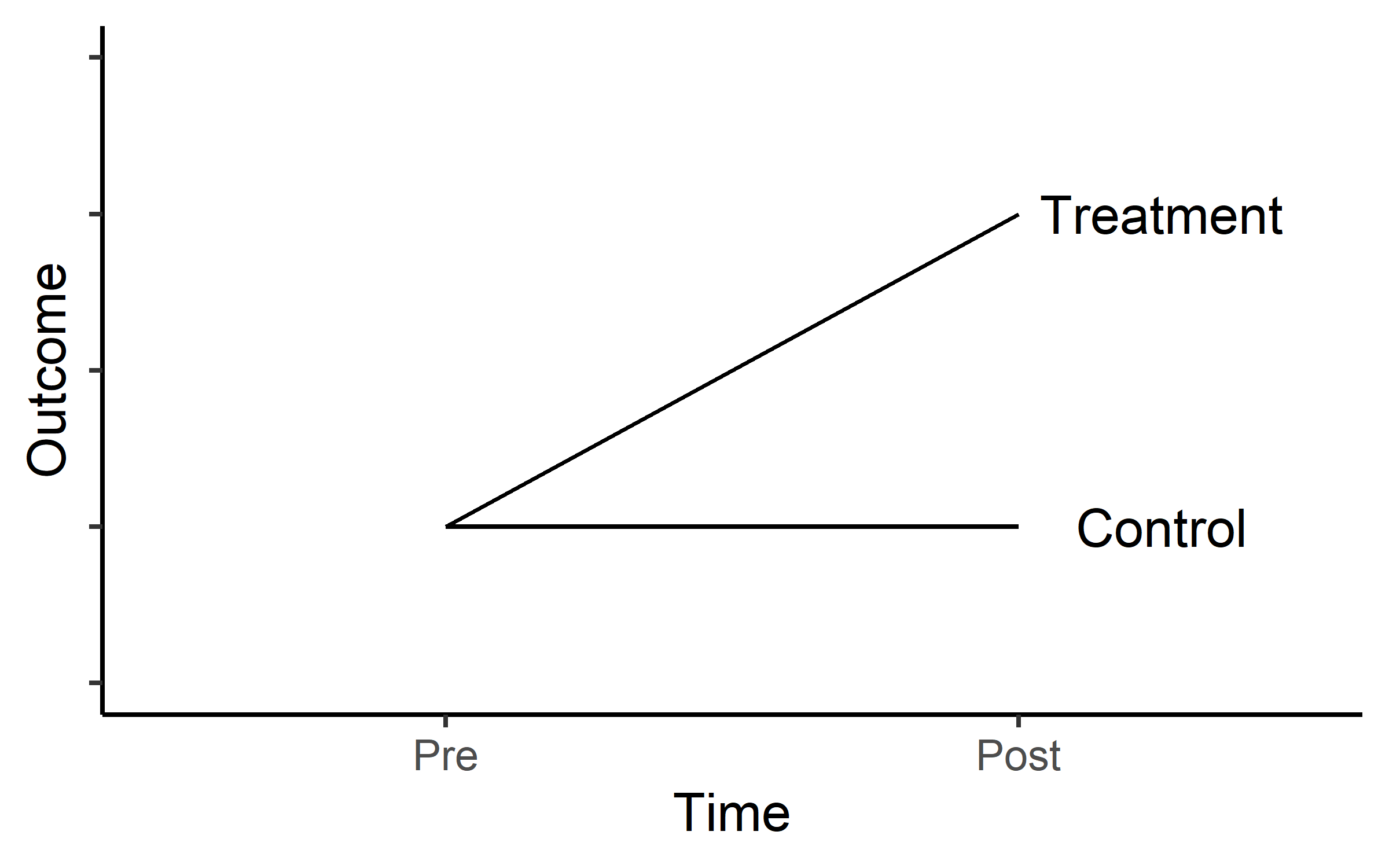
Figure 1.1: Hypothesized values from a simple pre-post parallel-groups design

Another common scenario is that we expect progress in two different treatments groups as in figure 1.2

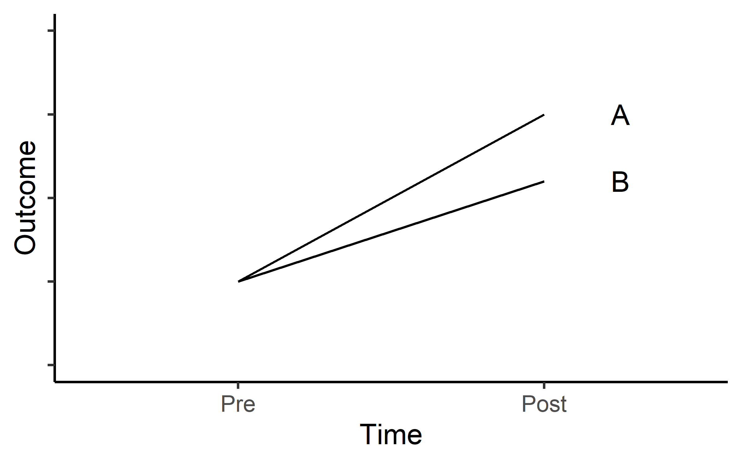
Figure 1.2: Hypothesized values from a simple pre-post parallel-groups design including to different treatments

In both scenarios we are interested in the treatment effect (or the difference in effect of two different treatments). This means that we want to establish if

\[ \Delta Y_A-\Delta Y_B \neq 0 \]

… meaning that the null hypothesis is that the change (\(\Delta\)) in group A is not different to the change in group B. To evaluate these studies we could do a t-test on the change score between groups. This is equivalent to a regression model where we model estimates the difference between groups

\[outcome = \beta_0 + \beta_1 Group_B\] In R, these to alternatives can be easily fitted using the code presented in code chunk (CC) 1:

# t.test example
with(data, t.test(outcome_A, outcome_B, paired = FALSE)

# The same in regression
lm(change ~ group, data = data)

This seemingly simple solution has some benefits but does not take into account that baseline values can affect the interpretation of a pre- to post-intervention study through regression to the mean. If we analyze change scores (\(post-pre\)), regression to the mean will give an overestimation of the effect, if there is, by chance, a difference in baseline values between groups (lower values in treatment group) (Vickers and Altman 2001a). If we analyze follow up scores (differences in post-scores between groups), the pattern will be reversed. To fix this problem we could control for the relationship between baseline values and the change scores. This technique is called Analysis of Co-Variance (ANCOVA), where the baseline is considered the added co-variance. This is an extension of the simple linear regression model (CC2).

# Extending the linear regression equation
lm(change ~ baseline + group, data = data)

We prefer the ANOCOVA model over the ordinary regression model as the ANCOVA model has better power (Senn 2006a). The ANCOVA model also gives unbiased estimates of differences between groups (Vickers and Altman 2001a). We can use the ANCOVA model when the allocation of participants have been done at random (e.g. RCTs) meaning that differences at baseline should be due to random variation.

2 Exercises: 10 vs 30RM-study

Thirty-one participants were assigned to one of two groups training with either 10 repetition maximum (RM) or 30RM, 27 participants completed the trials (24 participants completed to full time). The main question in the study was whether these two different treatments resulted in different magnitudes of strength development or muscle hypertrophy (we are interested in strength).

The file is available on canvas and contains the following variables:

1. subject: ID of participant
2. timepoint: prior to pre or after the intervention post
3. group: The intervention group
4. exercise: The exercise that was tested, legpress, benchpress or bicepscurl
5. load: The load lifted in 1RM test (kg)

An example of loading the data and plotting the data can be seen in CC3:

read_excel("./data/ten_vs_thirty.xlsx", na = "NA") %>%
        mutate(timepoint = factor(timepoint, 
                                  levels = c("pre", "mid", "post"))) %>%
        ggplot(aes(timepoint, load, fill = group)) + 
        geom_boxplot() +
        facet_wrap(~ exercise, scales = "free") + 
  theme_minimal()

The main purposo of our study is to answer the question: what training method would you recommend for improving maximal strength? To answer this question we will (1) Choose an appropriate 1RM test, (2) choose the most appropriate statistical model/test. To illustrate differences between models we will compare different models (lm on the change-score, lm with baseline as covariate, lm on post-values with baseline as a covariate).

2.1 Reducing the data set

For this exercise we will fous on the pre- to post-analysis of leg-press. To filter the data set we can use the code in CC4. We will have to re-shape the data for the calculation of change scores. We do this and add a simple calculation of change scores \(post-pre\).

ten_vs_thirty <- read_excel("./data/ten_vs_thirty.xlsx", na = "NA") %>%
  filter(timepoint != "mid", 
         exercise == "legpress") %>%
  # To get the variables in the correct order we need...
        mutate(timepoint = factor(timepoint, 
                                  levels = c("pre",  "post"))) %>% 
  pivot_wider(names_from = timepoint, 
              values_from = load) %>%
  mutate(change = post - pre) 

We are now ready to fit some models, these are outlined in CC5.

Before we look at the models, a word of caution: We should not select the model that best suit our hypothesis. Instead we should formulate a model that fits our question and intepret the results from a model that meets the assumptions of the analysis (homoscedasticity, normally distributed residuals etc.).

In this study it is reasonable to account for the baseline difference between groups. These differences are there because of the randomization. We may account for them by including them in our analysis (as in m2 and m4). To check if the addition of the baseline helps explain the data we can perform analysis of variance when comparing two models using the anova()-function.

The null hypothesis is that the addition of the pre variable does not help explain the observed variation in the data. Comparing model 1 and 2, and 3 and 4 (these have the same dependent variable) we see that there is strong evidence against the null hypothesis (CC6). In at least one case. The effect is not as clear in the other case but we could argue that this is evidence enough to include the variable as a calibrator.

To check if the models are well behaved we can use the plot function. Let’s first look at m1 comparing change score between groups.

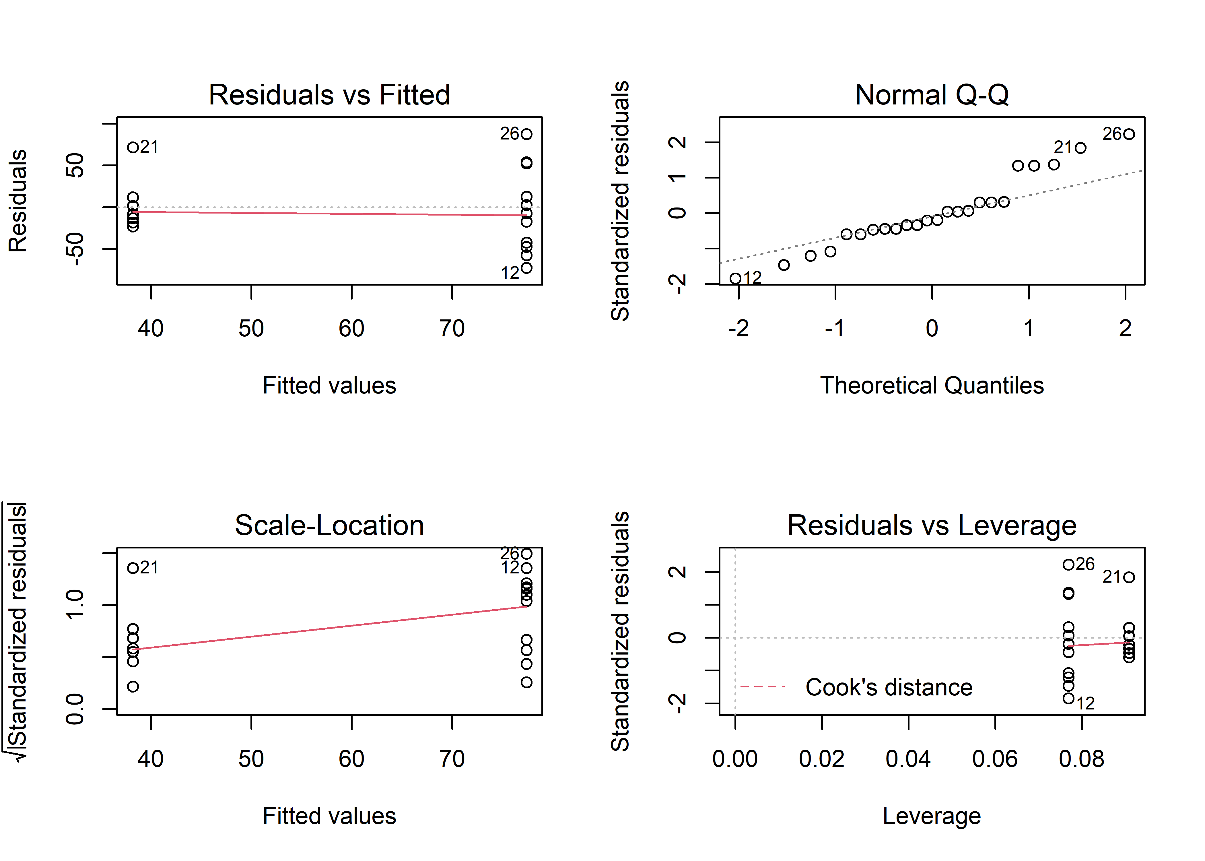
Figure 2.1: Diagnostic plots of Model 1

The plots in Figure 1.3 suggests that there is evidence of violation of the assumption of homoscedasticity (Residuals vs fitted, larger spread in higher fitted values also evident in the scale location plot). We can also see that the residuals are not normally distributed (Normal Q-Q plot). This model is not that good.

Let’s check the model with change between groups controlling for baseline values (Model 2). To create a similar grouped plot as above use the code in CC7

This is not a perfect model either, but the residuals looks a bit better. In fact the only model that would (almost) fail a more formal test is Model 1. The Brusch-Pagan test (see CC8) tests for heteroscedasticity. (This implies that a Welch t-test would be preferred (var.equal = FALSE))

2.2 Inference

Success! our models are somewhat OK. We may draw inference from them. It turns out that model modeling the change score or the post score does not matter when we control for the baseline. The difference between groups are exactly the same in Model 2 and 4 (CC9).

The pre variable changes as the relationship to the change is different to the relationship to post scores but the model does the same thing! This is now a question of how we would like to frame our question. If the question is “do people that train with 10RM increase their strength more than people that train with 30RM?” then model 2 is preferred. If the question is “are people who have trained with 10RM stronger than people who have trained with 30RM?” model 4 is preferred. The differences are basically semantics as the models tests the same thing, the differences between groups when controlling for baseline differences.

As we control for the baseline, we removes some of the unexplained error from the model, this will lead to a more powerful model. This is reflected in the stronger evidence (in a Fisherian way) against the null-hypothesis of no difference between groups.

2.3 What if the model diagnostics says the models are no good?

Biological data and performance data often exhibit larger variation at larger values. This leads to heteroscedasticity. A common way of dealing with this is the log transformation. Transforming the data to the log scale changes the interpretation of the regression coefficients.

# A linear model with the dependent variable on the linear scale!
m.linear <- lm(post ~ group + pre,  data = ten_vs_thirty)

# A linear model with the dependent variable on the log scale!
m.log <- lm(log(post) ~ group + pre,  data = ten_vs_thirty)

As we interpret the regression coefficients as differences the laws of the log are important to remember:

\[log(\frac{A}{B}) = log(A) - log(B)\] This means that the difference between two variables on the log scale is the same as the log of their quotient. When we back-transform values from the log scale we get the fold differences.

Let’s say that we have a mean in group A of 40 and a mean in group B of 20. The difference is 20. If we estimate the difference on the log scale however we will get (CC9):

a <- log(40/20)  

b <- log(40) - log(20)

c <- 40/20

exp(a)
exp(b)
c

The exp function back-transforms data from the log scale. Back-transforming a difference between two groups (as estimated in our model) will yield the fold-difference, this can be calculated as a percentage difference.

The 30RM group has a strength level 88% of the 10RM group at post, we can say that the 30RM group is 11% weaker than the 10RM group. Similarly, a confidence interval may also be back-transformed.

3 Exercises: Single vs. multiple sets

In this study, n = 34 participants were randomized to completed a strength training intervention with multiple-set and single-set randomized to either leg. Strength was evaluated as isokinetic strength at 60, 120 and 240 degrees and isometric strength, all using knee extension. In these exercises we will analyze data were participants have been selected either to belong to the single- or multiple-set group. This means we will only analyze one leg per participant!

3.1 The data set

The data can be found on canvas and contains six variables:

• subject
• timepoint (pre=Pre-training, session1=Pre-training second test, post=Post training)
• exercise (isok.60=Isokinetic 60 degrees per sec, isok.120, isok.240, isom=Isometric)
• load (Peak torque in Nm)
• sex (male, female)
• group (multiple, single)

The data can be found in strengthTests.csv on canvas. Use the read_csv() function (loaded in tidyverse) to load the data:

strength <- read_csv("./data/strengthTests.csv") %>%
  print()

3.2 Exploratory analysis

Use descriptive methods (summary statistics and figures to describe results from the trial). What are the mean and standard deviations of the load variable for each timepoint, exercise and group. Use tables and figures to show the results.

Here is a possible solution for a table

We want to summarize data per group, exercise and time-point and we want the means, standard deviations and the number of observations.

Here is a possible solution for a figure

Using the same summary statistics, we can create a figure. We might want to sort variables so that time-points are in the right order. In the figure we can use geom_errorbar to display SD

What can you say about the effect of single- vs. multiple-sets training on muscle strength using these observations?

3.3 Change from baseline

We will now focus on the change from baseline (pre) to the post time-point. To only use this data, use the filter function:

Calculate the average percentage change from baseline (pre) in each group and create a graph of the results. Focus on the isokinetic test performed at 120 degrees per second (isok.120). Make a plan of your code before you start writing it!

Here is a possible solution for a figure

Here we want to perform the following steps:

1. Filter the data to only contain pre and post time-points and exercise == "isok.120"
2. Make the data set wider and calculate percentage change as \(\frac{post-pre}{pre} \times 100\)
3. Group the data set by group and exercise
4. Summarize the data and create a figure with groups on the x-axis and %-change on the y-axis.

Example code

3.4 Model the change

The present data set is an example of a simple randomized trial. Participants have been randomized to either treatment before the trial and we are interested in the difference in treatments. There are several options for analyzing these data. A simple alternative would be to analyse the difference in post-training values with a t-test. This is not very efficient in terms of statistical power, i.e. we would need a lot of participants to show a difference if it existed due to differences between participants. In the case of the present data set, we have also collected more data than just follow-up scores. These baseline scores can be used to calculate a change-score which in turn can be used to compare treatments. This is a more direct comparison related to our actual question. We want to know what treatment is more effective in improving strength.

An example. We focus on the isok.120 data. State a hypothesis that compares the two groups and run a test that test against the corresponding null-hypothesis. Remember that we did this using both t.test() and lm(). Using var.equal = TRUE do the corresponding test also in lm. Write a short summary of your results!

Example code

3.5 Accounting for the baseline – Regression to the mean and extending the linear model

Above we created a linear model from where you got exactly the same results as from the t-test. In this section we will see that the linear model is easily extended to create more robust statistics of change scores.

When we have calculated a change score (e.g. percentage change), this score might be related to the baseline. This can be expected due to a phenomena known as regression towards the mean. When we do repeated testing on the same participants, test scores that were close to the upper or lower limit of a participant potential scores will be replaced with a score closer to the mean. This in turn will create a negative association between initial values and change.

Using the strength test data-set, calculate the change score using \(\frac{post-pre}{pre} *100\) and evaluate the association between change (y-axis) and baseline (x-axis) with a graph. Use + facte_wrap(~exercise, scales = "free") to get get a panel for each exercise.

How do you interpret the graphs?

Example code

read_csv("./data/strengthTests.csv") %>% 
        pivot_wider(names_from = timepoint, 
                    values_from = load) %>%
        mutate(change = (post-pre) / pre * 100) %>%
  ggplot(aes(pre, change)) + geom_point() + geom_smooth(method = "lm") + facet_wrap(~exercise, scales = "free")

An association between baseline and change scores means possible problems when we want to compare groups in the ordinary linear model. We can think of it in two ways. In the ordinary linear model (or the t-test of change scores) there is some unexplained variation that goes into the standard errors making it harder to see differences between groups. Taking the relationship into account creates a more powerful model. Secondly, there might be slight differences between groups in the baseline, when accounted for, we get an estimate of the difference between groups taking the baseline into account.

This extended model is called ANCOVA (ANalysis of CO-VAriance). The ordinary linear model we use above can be written as:

\[Change = \beta_0 + \beta_1 \times Group\]

The extended, ANCOVA model can be written as

\[Change = \beta_0 + \beta_1 \times Baseline + \beta_2 \times Group\]

In the following example we will use isom to infer on the effect of single- vs. multiple-set training. We will use the pre- to post training scores for change score calculations. In the data set we have men and women, to get an unbiased association to the baseline, we will mean center the pre-values per sex.

change.data <- read_csv("./data/strengthTests.csv") %>% 
        pivot_wider(names_from = timepoint, 
                    values_from = load) %>%
          mutate(change = (post-pre) / pre * 100) %>%
  group_by(sex) %>%
  mutate(pre = pre - mean(pre)) %>%
  filter(exercise == "isom") 


# An ordinary lm
m1 <- lm(change ~ group, data = change.data)

# An ancova
m2 <- lm(change ~ pre + group, data = change.data)

Side note: To get nice summaries of the model we will use kable() from the knitr package and tidy() from the broom package.

library(knitr); library(broom)

tidy(m1) %>%
  kable(col.names = c("Parameter", "Estimate", "SE", "t-statistic", "P-value"), 
        caption = "The ordinary linear model", digits = c(NA, 2, 2, 2, 3)) 

Table 3.1: The ordinary linear model

Parameter	Estimate	SE	t-statistic	P-value
(Intercept)	29.71	4.46	6.66	0.000
groupsingle	-11.51	6.22	-1.85	0.074

tidy(m2) %>%
  kable(col.names = c("Parameter", "Estimate", "SE", "t-statistic", "P-value"), 
        caption = "The ANCOVA model", digits = c(NA, 2, 2, 2, 3))

Table 3.1: The ANCOVA model

Parameter	Estimate	SE	t-statistic	P-value
(Intercept)	40.39	4.91	8.23	0.000
pre	-0.19	0.06	-3.48	0.002
groupsingle	-10.95	5.34	-2.05	0.049

In this case, modeling change-scores (percentage-change) together with the baseline makes a difference. We can be more confident on the results as some of the unexplained variation is cached in the association with the baseline.

We can use confidence intervals to see the estimates for the group effect:

data.frame(model = c("Linear-model", "ANCOVA"), 
           lower.CI = c(confint(m1)[2], confint(m2)[3]), 
           upper.CI = c(confint(m1)[4], confint(m2)[6])) %>%
  kable(col.names = c("Model", "Lower CI", "Upper CI"))

Model	Lower CI	Upper CI
Linear-model	-24.19385	1.1663784
ANCOVA	-21.85448	-0.0548598

These result will not repeat for all tests, but generally, the ANCOVA has more power and represents a good way of controlling for baseline measurements in change score analysis (Vickers and Altman 2001b; Senn 2006b).

3.6 Exercises

Perform an analysis of isok.120 data, infer on the effect of single- vs. multiple-sets on change in strength using the confidence intervals from an ANCOVA model. Remember to mean center the baseline per sex.

Example code

# Store the data set 

# Load data
change.data <- read_csv("./data/strengthTests.csv") %>% 
  # Pivot to a wide format for change calculation
        pivot_wider(names_from = timepoint, 
                    values_from = load) %>% 
  # Calculate the change
          mutate(change = (post-pre) / pre * 100) %>%
  # Mean center pre-variable with grouping on sex
  group_by(sex) %>%
  mutate(pre = pre - mean(pre)) %>%
  # Only use the isok.120 data
  filter(exercise == "isok.120") 



# Create the model
m1 <- lm(change ~ pre + group, data = change.data)

# Get confidence intervals
confint(m1)[c(3, 6)]

# Interpretation of the model 
summary(m1)

# The average %-change of the single-set group was ~5.6%-point lower than the multiple-set group. This effect was not significant on the 5% level. 

References

Senn, S. 2006a. “Change from Baseline and Analysis of Covariance Revisited.” Journal Article. Stat Med 25 (24): 4334–44. https://doi.org/10.1002/sim.2682.

———. 2006b. “Change from Baseline and Analysis of Covariance Revisited.” Journal Article. Stat Med 25 (24): 4334–44. https://doi.org/10.1002/sim.2682.

Vickers, Andrew J., and Douglas G. Altman. 2001a. “Analysing Controlled Trials with Baseline and Follow up Measurements.” Journal Article. BMJ : British Medical Journal 323 (7321): 1123–24. http://www.ncbi.nlm.nih.gov/pmc/articles/PMC1121605/ https://www.ncbi.nlm.nih.gov/pmc/articles/PMC1121605/pdf/1123.pdf.

———. 2001b. “Analysing Controlled Trials with Baseline and Follow up Measurements.” Journal Article. BMJ : British Medical Journal 323 (7321): 1123–24. http://www.ncbi.nlm.nih.gov/pmc/articles/PMC1121605/ https://www.ncbi.nlm.nih.gov/pmc/articles/PMC1121605/pdf/1123.pdf.