2  Before plotting

As we saw above, a basic visualization can be created from a dataset represented in R as a data frame, which is the most common representation of data in R. A tidy data set has one observation per row and one variable per column. A tidy data set makes data visualization easy. However, not all data sets are friendly. In fact, some might be unfriendly because they are unhappy¹.

A lot of effort goes into making data sets suitable for visualization or statistical modelling. The good news is that R is especially suited for the process of importing and wrangling data. As with other common tasks in R there are numerous ways of achieving the same goals. This is a good thing because it allows for solutions to a wide range of problems. It is also a bad thing because it makes it difficult to getting started. A collection of R packages called the Tidyverse makes the process of getting started with data wrangling easier.

Tidyverse can be thought of as a dialect of the R language. The dialect is designed to make it easy to write sequential operations in a way that translates thoughts and ideas to code. Sequential operations are enabled by a pipe operator. Using a pipe operator we can call functions in sequential order to do specific operations on the data. We can write such a pipe as demonstrated below with the corresponding English language descriptions to the left.

Take the data then do
filter the data based on x larger than 10 then do
add a new calculated variable z = x + y then do
show the output

data |>
  filter(x > 10) |>
  mutate(z = x + y) |>
  print()

The pipe operator (|>) takes any input and place it as the first argument in the following function². This is the mechanism that makes sequential operations possible. A pipe operator makes code more readable, consider the following two alternatives:

1print(mutate(filter(select(data, var1:var3), var1 == "xxx"), var4 = var1 + var2))


2data |>
  select(var1:var3) |>
  filter(var1 == "xxx") |>
  mutate(var4 = var1 + var2) 

1

Alternative 1: A number of operations are performed on data, we have to read from in to out to see each step.

2

Alternative 2: The same steps are performed as in alternative 1, in the same order.

The pipe in alternative 2 are structured with the pipe operator making the code more readable and easier to edit. Notice that the same functions are used in both cases.

In R there are two main pipe operators. We have the “base R” pipe, |>. This pipe operator is included in the base installation of R and available without loading any packages on start up. A second pipe belongs to the magritter package. The magritter pipe (%>%) has the same basic functionality as the base pipe; the left hand input is inserted as the first argument in any right hand function.

Sometimes you might want to place your input somewhere else than as the first argument in a right hand function. A placeholder can be used to indicate where you would like to place your input. The base pipe differs from the magritter pipe in what symbol indicates a placeholder. In the example below, the function some_fun() expects data as the third argument. We need to use our placeholder to put the data in the correct position:

1data |>
  some_fun(arg1 = c(1, 2), 
           arg2 = "some.setting", 
           arg3 = _)


library(tidyverse)
2data %>%
  some_fun(arg1 = c(1, 2), 
           arg2 = "some.setting", 
           arg3 = .)

1

With the base R forward pipe operator.

2

With the magritter forward pipe operator.

2.0.1 Reading data into R

Three packages makes reading tabular data into R easy. readr provides functions for reading and writing delimiter separated files, such as .csv or .tsv. readxl provides functions that imports data from excel files. An finally, googlesheets4 makes it possible to read tabular data created in google sheets.

Data can also be loaded from packages in R since storing data is a convenient way of sharing. By including data in a package you are nudged to do some quality checks and document it. We will talk more about data packages in a later workshop.

2.0.2 The verbs of data wrangling

Once data is available in our workspace we will be able to wrangle it. In the examples below I will use a data set containing results from dual x-ray absorptiometry measurements available in the exscidata package. To install the exscidata package:

library(remotes)
install_github("dhammarstrom/exscidata")

The dplyrpackage provides a collection of verbs to facilitate wrangling. As mentioned above, “pipeable” functions takes a data frame as its first argument. This means that we can line up functions in sequential order using a pipe operator. In all verb functions, following the data argument follows a set of arguments that specifies what we wish to do with the data. The result of the operations performed by the function are returned as a data frame.

dplyr contains the following main data verbs:

• select
• rename
• relocate
• mutate
• filter
• arrange
• summarize

In addition, several helper function will aid our wrangling endeavors.

dplyr is loaded as part of the tidyverse package:

library(tidyverse)

2.0.2.1 Select, rename and relocate variables

Variables in a data frame may be selected and renamed. Such operation may have multiple purposes such as giving you a better overview of the data of interest or limiting what data to display in a table. Renaming can make life easier if the data set contains long variable names.

Below we will store a subset of the data in a new data set. But we will first have a look at what column names are available:

1library(exscidata)
2glimpse(exscidata::dxadata)

1

Loading the exscidata package

2

Using glimbse we will get a overview of all available variables in the data set. The double :: means that we are looking for the data set dxadata inside the package exscidata.

Rows: 80
Columns: 59
$ participant      <chr> "FP28", "FP40", "FP21", "FP34", "FP23", "FP26", "FP36…
$ time             <chr> "pre", "pre", "pre", "pre", "pre", "pre", "pre", "pre…
$ multiple         <chr> "L", "R", "R", "R", "R", "R", "L", "R", "R", "L", "L"…
$ single           <chr> "R", "L", "L", "L", "L", "L", "R", "L", "L", "R", "R"…
$ sex              <chr> "female", "female", "male", "female", "male", "female…
$ include          <chr> "incl", "incl", "incl", "incl", "incl", "excl", "incl…
$ age              <dbl> 24.5, 22.1, 26.8, 23.1, 24.8, 24.2, 20.5, 20.6, 37.4,…
$ height           <dbl> 170.0, 175.0, 184.0, 164.0, 176.5, 163.0, 158.0, 181.…
$ weight           <dbl> 66.5, 64.0, 85.0, 53.0, 68.5, 56.0, 60.5, 83.5, 65.0,…
$ BMD.head         <dbl> 2.477, 1.916, 2.306, 2.163, 2.108, 2.866, 1.849, 2.21…
$ BMD.arms         <dbl> 0.952, 0.815, 0.980, 0.876, 0.917, 0.973, 0.871, 0.91…
$ BMD.legs         <dbl> 1.430, 1.218, 1.598, 1.256, 1.402, 1.488, 1.372, 1.42…
$ BMD.body         <dbl> 1.044, 0.860, 1.060, 0.842, 0.925, 0.984, 0.923, 1.01…
$ BMD.ribs         <dbl> 0.770, 0.630, 0.765, 0.636, 0.721, 0.737, 0.648, 0.70…
$ BMD.pelvis       <dbl> 1.252, 1.078, 1.314, 1.044, 1.154, 1.221, 1.194, 1.32…
$ BMD.spine        <dbl> 1.316, 0.979, 1.293, 0.899, 1.047, 1.089, 1.006, 1.14…
$ BMD.whole        <dbl> 1.268, 1.082, 1.325, 1.119, 1.181, 1.350, 1.166, 1.24…
$ fat.left_arm     <dbl> 1168, 715, 871, 610, 788, 372, 932, 1312, 388, 668, 5…
$ fat.left_leg     <dbl> 4469, 4696, 3467, 3023, 3088, 2100, 4674, 5435, 1873,…
$ fat.left_body    <dbl> 6280, 4061, 7740, 3638, 6018, 2328, 4896, 9352, 2921,…
$ fat.left_whole   <dbl> 12365, 9846, 12518, 7565, 10259, 5048, 10736, 16499, …
$ fat.right_arm    <dbl> 1205, 769, 871, 610, 741, 374, 940, 1292, 413, 716, 5…
$ fat.right_leg    <dbl> 4497, 4900, 3444, 3017, 3254, 2082, 4756, 5455, 1782,…
$ fat.right_body   <dbl> 6082, 3923, 8172, 3602, 5699, 2144, 4705, 8674, 2640,…
$ fat.right_whole  <dbl> 12102, 9862, 12856, 7479, 10020, 4821, 10806, 15876, …
$ fat.arms         <dbl> 2373, 1484, 1742, 1220, 1529, 747, 1872, 2604, 802, 1…
$ fat.legs         <dbl> 8965, 9596, 6911, 6040, 6342, 4182, 9430, 10890, 3655…
$ fat.body         <dbl> 12362, 7984, 15912, 7239, 11717, 4472, 9601, 18026, 5…
$ fat.android      <dbl> 1880, 963, 2460, 1203, 1933, 527, 1663, 3183, 1240, 1…
$ fat.gynoid       <dbl> 5064, 5032, 4779, 3739, 4087, 2740, 5217, 6278, 2309,…
$ fat.whole        <dbl> 24467, 19708, 25374, 15044, 20278, 9869, 21542, 32375…
$ lean.left_arm    <dbl> 1987, 1931, 2884, 1753, 2652, 2425, 1913, 2266, 3066,…
$ lean.left_leg    <dbl> 7059, 7190, 10281, 6014, 8242, 7903, 6829, 8889, 9664…
$ lean.left_body   <dbl> 9516, 10693, 13847, 9736, 11387, 10573, 8954, 11482, …
$ lean.left_whole  <dbl> 20305, 21778, 29332, 19143, 24185, 22946, 18809, 2431…
$ lean.right_arm   <dbl> 2049, 2081, 2888, 1754, 2487, 2439, 1930, 2236, 3253,…
$ lean.right_leg   <dbl> 7104, 7506, 10200, 6009, 8685, 7841, 6950, 8923, 9198…
$ lean.right_body  <dbl> 9199, 10304, 14593, 9636, 10779, 9733, 8602, 10672, 1…
$ lean.right_whole <dbl> 19605, 21310, 29643, 18792, 23653, 21837, 19407, 2372…
$ lean.arms        <dbl> 4036, 4012, 5773, 3508, 5139, 4864, 3843, 4501, 6319,…
$ lean.legs        <dbl> 14163, 14696, 20482, 12023, 16928, 15744, 13779, 1781…
$ lean.body        <dbl> 18715, 20998, 28440, 19372, 22166, 20306, 17556, 2215…
$ lean.android     <dbl> 2669, 2782, 3810, 2455, 2904, 2656, 2297, 3094, 3344,…
$ lean.gynoid      <dbl> 6219, 7209, 10233, 5866, 7525, 5970, 5825, 8175, 7760…
$ lean.whole       <dbl> 39910, 43088, 58976, 37934, 47837, 44783, 38216, 4804…
$ BMC.left_arm     <dbl> 181, 138, 204, 144, 180, 173, 140, 173, 220, 226, 225…
$ BMC.left_leg     <dbl> 567, 508, 728, 441, 562, 574, 482, 631, 633, 630, 672…
$ BMC.left_body    <dbl> 622, 414, 696, 367, 526, 465, 370, 629, 473, 629, 509…
$ BMC.left_whole   <dbl> 1680, 1321, 1945, 1201, 1527, 1580, 1131, 1688, 1544,…
$ BMC.right_arm    <dbl> 198, 150, 210, 142, 176, 183, 140, 176, 224, 251, 226…
$ BMC.right_leg    <dbl> 574, 514, 739, 431, 552, 565, 491, 641, 622, 636, 690…
$ BMC.right_body   <dbl> 592, 428, 730, 351, 502, 409, 358, 582, 420, 616, 483…
$ BMC.right_whole  <dbl> 1582, 1288, 1958, 1130, 1451, 1466, 1229, 1668, 1478,…
$ BMC.arms         <dbl> 379, 288, 414, 285, 356, 357, 280, 348, 444, 478, 451…
$ BMC.legs         <dbl> 1142, 1022, 1467, 872, 1115, 1139, 974, 1272, 1255, 1…
$ BMC.body         <dbl> 1214, 842, 1426, 718, 1028, 874, 728, 1211, 893, 1245…
$ BMC.android      <dbl> 80, 57, 90, 44, 56, 54, 43, 77, 52, 72, 59, 60, 65, 5…
$ BMC.gynoid       <dbl> 314, 285, 427, 245, 299, 262, 241, 379, 335, 378, 332…
$ BMC.whole        <dbl> 3261, 2609, 3903, 2331, 2978, 3046, 2360, 3356, 3022,…

The data set contains 80 rows and 59 columns. The variables in the data set are described as part of the exscidata package and can be seen by typing ?dxadata in the console.

We will work further with lean body mass data, these are variables starting with lean.. In addition we need variables describing observations like participant, time, multiple, single, sex, include, height and weight. To select these variables we can try a couple of different approaches. The select function can select variables by name. This means that we can simply list them:

1exscidata::dxadata |>
2  select(participant, time, multiple, single) |>
3  print()

1

Retrieve the data from the exscidata package

2

select variables based on names

3

Print the resulting data frame.

# A tibble: 80 × 4
   participant time  multiple single
   <chr>       <chr> <chr>    <chr> 
 1 FP28        pre   L        R     
 2 FP40        pre   R        L     
 3 FP21        pre   R        L     
 4 FP34        pre   R        L     
 5 FP23        pre   R        L     
 6 FP26        pre   R        L     
 7 FP36        pre   L        R     
 8 FP38        pre   R        L     
 9 FP25        pre   R        L     
10 FP19        pre   L        R     
# ℹ 70 more rows

The above approach means a lot of work writing all columns names in the select call. An alternative approach is to select variables based on the first and last variable in a sequence. This is possible by using the syntax <first column>:<last column>.

exscidata::dxadata |>  
1  select(participant:weight) |>
  print() 

1

Selecting by the first and last column in a sequence.

# A tibble: 80 × 9
   participant time  multiple single sex    include   age height weight
   <chr>       <chr> <chr>    <chr>  <chr>  <chr>   <dbl>  <dbl>  <dbl>
 1 FP28        pre   L        R      female incl     24.5   170    66.5
 2 FP40        pre   R        L      female incl     22.1   175    64  
 3 FP21        pre   R        L      male   incl     26.8   184    85  
 4 FP34        pre   R        L      female incl     23.1   164    53  
 5 FP23        pre   R        L      male   incl     24.8   176.   68.5
 6 FP26        pre   R        L      female excl     24.2   163    56  
 7 FP36        pre   L        R      female incl     20.5   158    60.5
 8 FP38        pre   R        L      female incl     20.6   181    83.5
 9 FP25        pre   R        L      male   incl     37.4   183    65  
10 FP19        pre   L        R      male   incl     22.3   178.   73.5
# ℹ 70 more rows

We also like to have the lean body mass data included in our new data set. Since all variables containing lean body mass data starts with lean. we can use a helper function to select them. Two alternatives are possible:

exscidata::dxadata |>  
1  select(participant:weight, starts_with("lean.")) |>
  print() 


exscidata::dxadata |>  
2  select(participant:weight, contains("lean.")) |>
  print() 

1

Using starts_with to select all columns that starts with lean.

2

Using containsto select all variables that contains lean.

# A tibble: 80 × 23
   participant time  multiple single sex    include   age height weight
   <chr>       <chr> <chr>    <chr>  <chr>  <chr>   <dbl>  <dbl>  <dbl>
 1 FP28        pre   L        R      female incl     24.5   170    66.5
 2 FP40        pre   R        L      female incl     22.1   175    64  
 3 FP21        pre   R        L      male   incl     26.8   184    85  
 4 FP34        pre   R        L      female incl     23.1   164    53  
 5 FP23        pre   R        L      male   incl     24.8   176.   68.5
 6 FP26        pre   R        L      female excl     24.2   163    56  
 7 FP36        pre   L        R      female incl     20.5   158    60.5
 8 FP38        pre   R        L      female incl     20.6   181    83.5
 9 FP25        pre   R        L      male   incl     37.4   183    65  
10 FP19        pre   L        R      male   incl     22.3   178.   73.5
# ℹ 70 more rows
# ℹ 14 more variables: lean.left_arm <dbl>, lean.left_leg <dbl>,
#   lean.left_body <dbl>, lean.left_whole <dbl>, lean.right_arm <dbl>,
#   lean.right_leg <dbl>, lean.right_body <dbl>, lean.right_whole <dbl>,
#   lean.arms <dbl>, lean.legs <dbl>, lean.body <dbl>, lean.android <dbl>,
#   lean.gynoid <dbl>, lean.whole <dbl>
# A tibble: 80 × 23
   participant time  multiple single sex    include   age height weight
   <chr>       <chr> <chr>    <chr>  <chr>  <chr>   <dbl>  <dbl>  <dbl>
 1 FP28        pre   L        R      female incl     24.5   170    66.5
 2 FP40        pre   R        L      female incl     22.1   175    64  
 3 FP21        pre   R        L      male   incl     26.8   184    85  
 4 FP34        pre   R        L      female incl     23.1   164    53  
 5 FP23        pre   R        L      male   incl     24.8   176.   68.5
 6 FP26        pre   R        L      female excl     24.2   163    56  
 7 FP36        pre   L        R      female incl     20.5   158    60.5
 8 FP38        pre   R        L      female incl     20.6   181    83.5
 9 FP25        pre   R        L      male   incl     37.4   183    65  
10 FP19        pre   L        R      male   incl     22.3   178.   73.5
# ℹ 70 more rows
# ℹ 14 more variables: lean.left_arm <dbl>, lean.left_leg <dbl>,
#   lean.left_body <dbl>, lean.left_whole <dbl>, lean.right_arm <dbl>,
#   lean.right_leg <dbl>, lean.right_body <dbl>, lean.right_whole <dbl>,
#   lean.arms <dbl>, lean.legs <dbl>, lean.body <dbl>, lean.android <dbl>,
#   lean.gynoid <dbl>, lean.whole <dbl>

There are other select helper functions such as ends_with and matches that work in a similar fashion as the above. all_of and any_of helps you select variables based on a vector of variables, where selects based on where a function of your choosing returns true. See ?select for a complete list.

In a select call we can also rename variables using the syntax <new name> = <old name>. Let’s say we want to select and rename participant:

exscidata::dxadata |>  
  select(parti = participant, time:weight, starts_with("lean.")) |> 
  print() 

# A tibble: 80 × 23
   parti time  multiple single sex    include   age height weight lean.left_arm
   <chr> <chr> <chr>    <chr>  <chr>  <chr>   <dbl>  <dbl>  <dbl>         <dbl>
 1 FP28  pre   L        R      female incl     24.5   170    66.5          1987
 2 FP40  pre   R        L      female incl     22.1   175    64            1931
 3 FP21  pre   R        L      male   incl     26.8   184    85            2884
 4 FP34  pre   R        L      female incl     23.1   164    53            1753
 5 FP23  pre   R        L      male   incl     24.8   176.   68.5          2652
 6 FP26  pre   R        L      female excl     24.2   163    56            2425
 7 FP36  pre   L        R      female incl     20.5   158    60.5          1913
 8 FP38  pre   R        L      female incl     20.6   181    83.5          2266
 9 FP25  pre   R        L      male   incl     37.4   183    65            3066
10 FP19  pre   L        R      male   incl     22.3   178.   73.5          3760
# ℹ 70 more rows
# ℹ 13 more variables: lean.left_leg <dbl>, lean.left_body <dbl>,
#   lean.left_whole <dbl>, lean.right_arm <dbl>, lean.right_leg <dbl>,
#   lean.right_body <dbl>, lean.right_whole <dbl>, lean.arms <dbl>,
#   lean.legs <dbl>, lean.body <dbl>, lean.android <dbl>, lean.gynoid <dbl>,
#   lean.whole <dbl>

Notice how different ways of selecting variables can be combined in select.

The rename function makes it easy to rename variables without the need to select.

exscidata::dxadata |>  
  select(participant:weight, starts_with("lean.")) |> 
  rename(parti = participant) |>
  print() 

# A tibble: 80 × 23
   parti time  multiple single sex    include   age height weight lean.left_arm
   <chr> <chr> <chr>    <chr>  <chr>  <chr>   <dbl>  <dbl>  <dbl>         <dbl>
 1 FP28  pre   L        R      female incl     24.5   170    66.5          1987
 2 FP40  pre   R        L      female incl     22.1   175    64            1931
 3 FP21  pre   R        L      male   incl     26.8   184    85            2884
 4 FP34  pre   R        L      female incl     23.1   164    53            1753
 5 FP23  pre   R        L      male   incl     24.8   176.   68.5          2652
 6 FP26  pre   R        L      female excl     24.2   163    56            2425
 7 FP36  pre   L        R      female incl     20.5   158    60.5          1913
 8 FP38  pre   R        L      female incl     20.6   181    83.5          2266
 9 FP25  pre   R        L      male   incl     37.4   183    65            3066
10 FP19  pre   L        R      male   incl     22.3   178.   73.5          3760
# ℹ 70 more rows
# ℹ 13 more variables: lean.left_leg <dbl>, lean.left_body <dbl>,
#   lean.left_whole <dbl>, lean.right_arm <dbl>, lean.right_leg <dbl>,
#   lean.right_body <dbl>, lean.right_whole <dbl>, lean.arms <dbl>,
#   lean.legs <dbl>, lean.body <dbl>, lean.android <dbl>, lean.gynoid <dbl>,
#   lean.whole <dbl>

If we want to change the order of variables in a data set we can specify the order in a select call, or use relocate

exscidata::dxadata |>  
  select(participant:weight, starts_with("lean.")) |> 
  relocate(lean.whole) |>
  print() 

# A tibble: 80 × 23
   lean.whole participant time  multiple single sex    include   age height
        <dbl> <chr>       <chr> <chr>    <chr>  <chr>  <chr>   <dbl>  <dbl>
 1      39910 FP28        pre   L        R      female incl     24.5   170 
 2      43088 FP40        pre   R        L      female incl     22.1   175 
 3      58976 FP21        pre   R        L      male   incl     26.8   184 
 4      37934 FP34        pre   R        L      female incl     23.1   164 
 5      47837 FP23        pre   R        L      male   incl     24.8   176.
 6      44783 FP26        pre   R        L      female excl     24.2   163 
 7      38216 FP36        pre   L        R      female incl     20.5   158 
 8      48045 FP38        pre   R        L      female incl     20.6   181 
 9      54710 FP25        pre   R        L      male   incl     37.4   183 
10      58740 FP19        pre   L        R      male   incl     22.3   178.
# ℹ 70 more rows
# ℹ 14 more variables: weight <dbl>, lean.left_arm <dbl>, lean.left_leg <dbl>,
#   lean.left_body <dbl>, lean.left_whole <dbl>, lean.right_arm <dbl>,
#   lean.right_leg <dbl>, lean.right_body <dbl>, lean.right_whole <dbl>,
#   lean.arms <dbl>, lean.legs <dbl>, lean.body <dbl>, lean.android <dbl>,
#   lean.gynoid <dbl>

relocate puts the selected variable as the first column in the data set. If we want to specify the location we can use the arguments .before or .after.

exscidata::dxadata |>  
  select(participant:weight, starts_with("lean.")) |> 
  relocate(lean.whole, .after = sex) |>
  print() 

# A tibble: 80 × 23
   participant time  multiple single sex    lean.whole include   age height
   <chr>       <chr> <chr>    <chr>  <chr>       <dbl> <chr>   <dbl>  <dbl>
 1 FP28        pre   L        R      female      39910 incl     24.5   170 
 2 FP40        pre   R        L      female      43088 incl     22.1   175 
 3 FP21        pre   R        L      male        58976 incl     26.8   184 
 4 FP34        pre   R        L      female      37934 incl     23.1   164 
 5 FP23        pre   R        L      male        47837 incl     24.8   176.
 6 FP26        pre   R        L      female      44783 excl     24.2   163 
 7 FP36        pre   L        R      female      38216 incl     20.5   158 
 8 FP38        pre   R        L      female      48045 incl     20.6   181 
 9 FP25        pre   R        L      male        54710 incl     37.4   183 
10 FP19        pre   L        R      male        58740 incl     22.3   178.
# ℹ 70 more rows
# ℹ 14 more variables: weight <dbl>, lean.left_arm <dbl>, lean.left_leg <dbl>,
#   lean.left_body <dbl>, lean.left_whole <dbl>, lean.right_arm <dbl>,
#   lean.right_leg <dbl>, lean.right_body <dbl>, lean.right_whole <dbl>,
#   lean.arms <dbl>, lean.legs <dbl>, lean.body <dbl>, lean.android <dbl>,
#   lean.gynoid <dbl>

2.0.2.2 Creating new variables

mutate let’s us create new variables in a data set. These can be a function of variables already in the data set or created from our input.

Let’s create a variable representing the percentage of lean mass to body mass.

exscidata::dxadata |>  
  select(participant:weight, starts_with("lean.")) |> 
  mutate(rel_lean_whole = 100 * ((lean.whole/1000) / weight)) |>
  relocate(rel_lean_whole) |>
  print() 

# A tibble: 80 × 24
   rel_lean_whole participant time  multiple single sex    include   age height
            <dbl> <chr>       <chr> <chr>    <chr>  <chr>  <chr>   <dbl>  <dbl>
 1           60.0 FP28        pre   L        R      female incl     24.5   170 
 2           67.3 FP40        pre   R        L      female incl     22.1   175 
 3           69.4 FP21        pre   R        L      male   incl     26.8   184 
 4           71.6 FP34        pre   R        L      female incl     23.1   164 
 5           69.8 FP23        pre   R        L      male   incl     24.8   176.
 6           80.0 FP26        pre   R        L      female excl     24.2   163 
 7           63.2 FP36        pre   L        R      female incl     20.5   158 
 8           57.5 FP38        pre   R        L      female incl     20.6   181 
 9           84.2 FP25        pre   R        L      male   incl     37.4   183 
10           79.9 FP19        pre   L        R      male   incl     22.3   178.
# ℹ 70 more rows
# ℹ 15 more variables: weight <dbl>, lean.left_arm <dbl>, lean.left_leg <dbl>,
#   lean.left_body <dbl>, lean.left_whole <dbl>, lean.right_arm <dbl>,
#   lean.right_leg <dbl>, lean.right_body <dbl>, lean.right_whole <dbl>,
#   lean.arms <dbl>, lean.legs <dbl>, lean.body <dbl>, lean.android <dbl>,
#   lean.gynoid <dbl>, lean.whole <dbl>

2.0.3 From wide to long and back again

The dxadata data set is not a tidy data set. It contains two variables (single and multiple) that indicates which leg has been training with low and moderate volume respectively (Hammarström et al. 2020). Additionally, lean mass variables could be separated based on body half (right or left). To compare training volume we need to reformat the data set. We will start by making a smaller data set that indicate training volume per leg.

As we have already seen, participant, single and multiple are the variables needed to make a data set that indicates training volume per leg, per participant. We will start by selecting these columns followed by pivoting the data as the volume data is located in two variables. This essentially means that we will make the data set longer.

exscidata::dxadata |>  
1  select(participant, multiple, single) |>
2  pivot_longer(values_to = "leg", names_to = "volume",  cols = multiple:single) %>%
  print()

1

Selecting our variables of interest

2

Creating a long data set based on volume data spread over two columns.

# A tibble: 160 × 3
   participant volume   leg  
   <chr>       <chr>    <chr>
 1 FP28        multiple L    
 2 FP28        single   R    
 3 FP40        multiple R    
 4 FP40        single   L    
 5 FP21        multiple R    
 6 FP21        single   L    
 7 FP34        multiple R    
 8 FP34        single   L    
 9 FP23        multiple R    
10 FP23        single   L    
# ℹ 150 more rows

As we see we now have a long data set, but it is longer than expected. The original data contains only 41 participants. As each participant has two legs we would expect 82 observations. Above we did not remove post-intervention observations and we therefore have several duplicates. This can be taken care of by using the distinct function which returns unique observations across a combination of variables.

participant_volume <- exscidata::dxadata |>  
  select(participant, multiple, single) |> # 
  pivot_longer(values_to = "leg", names_to = "volume",  cols = multiple:single) %>%
1  distinct(participant, volume, leg) %>%
  print()

1

Removes all duplicate combinations of participant, volume and leg.

# A tibble: 82 × 3
   participant volume   leg  
   <chr>       <chr>    <chr>
 1 FP28        multiple L    
 2 FP28        single   R    
 3 FP40        multiple R    
 4 FP40        single   L    
 5 FP21        multiple R    
 6 FP21        single   L    
 7 FP34        multiple R    
 8 FP34        single   L    
 9 FP23        multiple R    
10 FP23        single   L    
# ℹ 72 more rows

We can save our smaller data set as participant_volume

Next we want to create a data set of right and left leg lean mass data. We will start by selecting variables.

exscidata::dxadata |>  
  select(participant, time, starts_with("lean.") & ends_with("_leg")) |> #
  print()

# A tibble: 80 × 4
   participant time  lean.left_leg lean.right_leg
   <chr>       <chr>         <dbl>          <dbl>
 1 FP28        pre            7059           7104
 2 FP40        pre            7190           7506
 3 FP21        pre           10281          10200
 4 FP34        pre            6014           6009
 5 FP23        pre            8242           8685
 6 FP26        pre            7903           7841
 7 FP36        pre            6829           6950
 8 FP38        pre            8889           8923
 9 FP25        pre            9664           9198
10 FP19        pre            9704           9806
# ℹ 70 more rows

Notice how & was used to create a conditional selection of variables. I addition to selecting time, include³ and participant we select variables that starts with lean. AND ends with _leg.

The resulting data set is wide. Two variables contains the same variable (lean mass), but one variable (leg) is lurking in two variables (lean.left_leg and lean.right_leg). Let’s make the data set long.

3leg_leanmass <- exscidata::dxadata |>
  select(participant, time, include, starts_with("lean.") & ends_with("_leg")) |> 
1  pivot_longer(names_to = "leg", values_to = "lean_mass", cols = contains("lean.")) |>
2  mutate(leg = if_else(leg == "lean.left_leg", "L", "R")) |>
  
  print()

1

Notice how select helpers can be used in pivot_longer.

2

We use mutate together with if_else to change the leg indicator to R and L

3

We save the data set as leg_leanmass

# A tibble: 160 × 5
   participant time  include leg   lean_mass
   <chr>       <chr> <chr>   <chr>     <dbl>
 1 FP28        pre   incl    L          7059
 2 FP28        pre   incl    R          7104
 3 FP40        pre   incl    L          7190
 4 FP40        pre   incl    R          7506
 5 FP21        pre   incl    L         10281
 6 FP21        pre   incl    R         10200
 7 FP34        pre   incl    L          6014
 8 FP34        pre   incl    R          6009
 9 FP23        pre   incl    L          8242
10 FP23        pre   incl    R          8685
# ℹ 150 more rows

pivot_longer has a brother called pivot_wider, this functions performs the reverse operation making long data sets wide. Let’s say that we would like to calculate the paired difference of leg lean mass from pre to post, we could make a wider data set and calculate post - pre

exscidata::dxadata |>  
  select(participant, time, include, starts_with("lean.") & ends_with("_leg")) |> 
  pivot_longer(names_to = "leg", values_to = "lean_mass", cols = contains("lean.")) |>
  mutate(leg = if_else(leg == "lean.left_leg", "L", "R")) |> 
1  pivot_wider(names_from = time, values_from = lean_mass) |>
2  mutate(delta_lean_mass = post - pre) |>
  print()

1

Pivot wider creates new columns based on names in time and values in lean_mass

2

The new variables is calculated as the difference between pre and post-intervention values.

# A tibble: 82 × 6
   participant include leg     pre  post delta_lean_mass
   <chr>       <chr>   <chr> <dbl> <dbl>           <dbl>
 1 FP28        incl    L      7059  7273             214
 2 FP28        incl    R      7104  7227             123
 3 FP40        incl    L      7190  7192               2
 4 FP40        incl    R      7506  7437             -69
 5 FP21        incl    L     10281 10470             189
 6 FP21        incl    R     10200 10819             619
 7 FP34        incl    L      6014  6326             312
 8 FP34        incl    R      6009  6405             396
 9 FP23        incl    L      8242  8687             445
10 FP23        incl    R      8685  8480            -205
# ℹ 72 more rows

2.0.4 Joining data sets

We have constructed two smaller data sets, one indicating which leg performed low and moderate volume and one data set containing the lean mass values for each leg, pre- and post-intervention. Next step is to join the two.

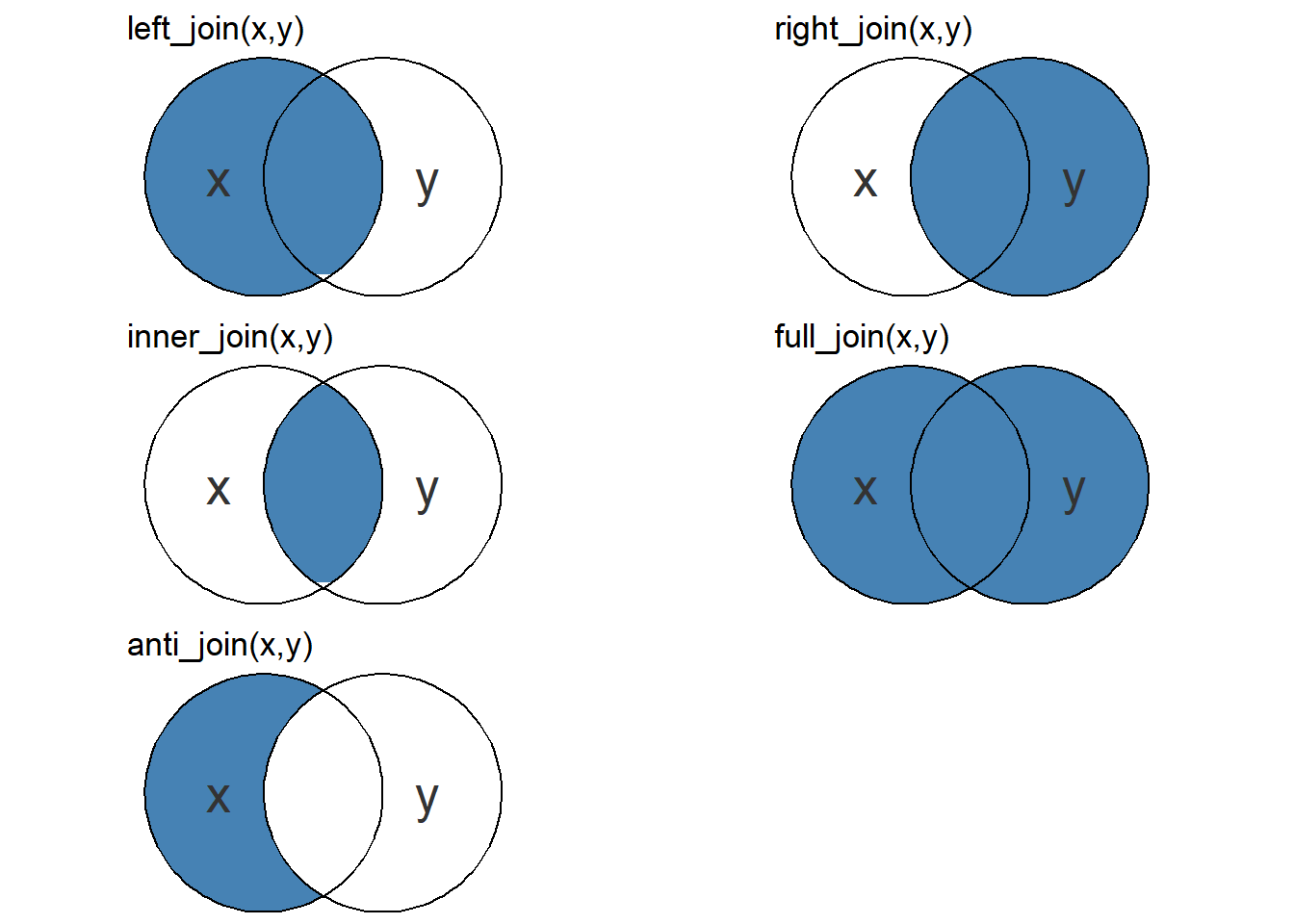
dplyr contains functions for joining data frames. There are, as illustrated in Figure 2.1 important differences between the functions where outer joins (left, right and full) keeps all observations in x, y and both x and y respectively. inner_join however, drops unmatched observations from both input data frames. Unlike the others, anti_join function removes observations in x that is present in y.

Figure 2.1: Functions for joining data sets.

Our two data sets are pretty insensitive to dropped observations since the two data sets should be complete. We will use a left_join to put the data set together. This will match participant and leg because these two variables exists in both data sets. If we want to join by other variables we may specify such a variable. We’ll save the joined data set as leg_leanmass.

leg_leanmass <- leg_leanmass |>
  inner_join(participant_volume) |>
  print()

Joining with `by = join_by(participant, leg)`

# A tibble: 160 × 6
   participant time  include leg   lean_mass volume  
   <chr>       <chr> <chr>   <chr>     <dbl> <chr>   
 1 FP28        pre   incl    L          7059 multiple
 2 FP28        pre   incl    R          7104 single  
 3 FP40        pre   incl    L          7190 single  
 4 FP40        pre   incl    R          7506 multiple
 5 FP21        pre   incl    L         10281 single  
 6 FP21        pre   incl    R         10200 multiple
 7 FP34        pre   incl    L          6014 single  
 8 FP34        pre   incl    R          6009 multiple
 9 FP23        pre   incl    L          8242 single  
10 FP23        pre   incl    R          8685 multiple
# ℹ 150 more rows

2.0.5 Filters and sorting rows

We included the variable include in our data set, this will make it possible to get rid of observations from participants that should be part of the final analysis. We can use filter to perform this operation.

leg_leanmass |>
  filter(include == "incl") |>
  print()

# A tibble: 136 × 6
   participant time  include leg   lean_mass volume  
   <chr>       <chr> <chr>   <chr>     <dbl> <chr>   
 1 FP28        pre   incl    L          7059 multiple
 2 FP28        pre   incl    R          7104 single  
 3 FP40        pre   incl    L          7190 single  
 4 FP40        pre   incl    R          7506 multiple
 5 FP21        pre   incl    L         10281 single  
 6 FP21        pre   incl    R         10200 multiple
 7 FP34        pre   incl    L          6014 single  
 8 FP34        pre   incl    R          6009 multiple
 9 FP23        pre   incl    L          8242 single  
10 FP23        pre   incl    R          8685 multiple
# ℹ 126 more rows

The double equal sign can be read as “equal to” in R, a common source of confusion is that the single equal sign (=) is used as a assignment operator.⁴

The filter function keeps rows of a data frame where a condition that we specify returns TRUE. To construct testable conditions that allows for results being either FALSE or TRUE we will use one, or a combination operators, such as

==	→ “equal to”
!=	→ “not equal to”
>	→ “larger than”
<	→ “smaller than”
>=, <=	→ “larger/smaller or equal to”
!	→ “NOT”
&	→ “AND”
|	→ “OR”

The above are all part of a collection of logical operators.⁵ We may demonstrate the mechanism by which filter operates by creating our own vector of TRUE/FALSE values. In the code chunk below a vector (INCLUDE) is created based on our include variable. A logical vector is created from the statement INCLUDE != "excl". We then use this vector in the filter statement.

INCLUDE <- leg_leanmass |>
  pull(include)

INCLUDE <- INCLUDE != "excl"


INCLUDE

  [1]  TRUE  TRUE  TRUE  TRUE  TRUE  TRUE  TRUE  TRUE  TRUE  TRUE FALSE FALSE
 [13]  TRUE  TRUE  TRUE  TRUE  TRUE  TRUE  TRUE  TRUE  TRUE  TRUE  TRUE  TRUE
 [25]  TRUE  TRUE  TRUE  TRUE  TRUE  TRUE  TRUE  TRUE  TRUE  TRUE  TRUE  TRUE
 [37]  TRUE  TRUE  TRUE  TRUE FALSE FALSE  TRUE  TRUE  TRUE  TRUE FALSE FALSE
 [49] FALSE FALSE FALSE FALSE  TRUE  TRUE  TRUE  TRUE  TRUE  TRUE  TRUE  TRUE
 [61]  TRUE  TRUE  TRUE  TRUE  TRUE  TRUE FALSE FALSE  TRUE  TRUE  TRUE  TRUE
 [73]  TRUE  TRUE FALSE FALSE  TRUE  TRUE  TRUE  TRUE  TRUE  TRUE  TRUE  TRUE
 [85]  TRUE  TRUE  TRUE  TRUE  TRUE  TRUE  TRUE  TRUE  TRUE  TRUE  TRUE  TRUE
 [97]  TRUE  TRUE  TRUE  TRUE  TRUE  TRUE  TRUE  TRUE  TRUE  TRUE  TRUE  TRUE
[109]  TRUE  TRUE  TRUE  TRUE  TRUE  TRUE  TRUE  TRUE FALSE FALSE  TRUE  TRUE
[121]  TRUE  TRUE  TRUE  TRUE  TRUE  TRUE  TRUE  TRUE  TRUE  TRUE  TRUE  TRUE
[133]  TRUE  TRUE  TRUE  TRUE  TRUE  TRUE  TRUE  TRUE  TRUE  TRUE  TRUE  TRUE
[145]  TRUE  TRUE FALSE FALSE  TRUE  TRUE FALSE FALSE  TRUE  TRUE  TRUE  TRUE
[157] FALSE FALSE FALSE FALSE

leg_leanmass |>
  filter(INCLUDE)

# A tibble: 136 × 6
   participant time  include leg   lean_mass volume  
   <chr>       <chr> <chr>   <chr>     <dbl> <chr>   
 1 FP28        pre   incl    L          7059 multiple
 2 FP28        pre   incl    R          7104 single  
 3 FP40        pre   incl    L          7190 single  
 4 FP40        pre   incl    R          7506 multiple
 5 FP21        pre   incl    L         10281 single  
 6 FP21        pre   incl    R         10200 multiple
 7 FP34        pre   incl    L          6014 single  
 8 FP34        pre   incl    R          6009 multiple
 9 FP23        pre   incl    L          8242 single  
10 FP23        pre   incl    R          8685 multiple
# ℹ 126 more rows

In R, a vector of TRUE/FALSE (or in short form T/F) are is a special case which R will prohibit us from overwriting.

2.0.5.1 Grouped filters

Using the dplyr syntax it is easy to e.g. filter or mutate based on a grouping of the data set. The function group_by creates a grouped data set. In the context of filtering in our data set we may want to filter out observations larger than the median from two time points.

leg_leanmass |>
  group_by(time) |>
  filter(lean_mass > median(lean_mass)) |> 
  print()

# A tibble: 80 × 6
# Groups:   time [2]
   participant time  include leg   lean_mass volume  
   <chr>       <chr> <chr>   <chr>     <dbl> <chr>   
 1 FP21        pre   incl    L         10281 single  
 2 FP21        pre   incl    R         10200 multiple
 3 FP23        pre   incl    R          8685 multiple
 4 FP38        pre   incl    L          8889 single  
 5 FP38        pre   incl    R          8923 multiple
 6 FP25        pre   incl    L          9664 single  
 7 FP25        pre   incl    R          9198 multiple
 8 FP19        pre   incl    L          9704 multiple
 9 FP19        pre   incl    R          9806 single  
10 FP13        pre   incl    L         10086 multiple
# ℹ 70 more rows

The above operation removed exactly half of the observations, as expected since we wanted observations larger than the median from both time points. We may combine this statement with filtering away "excl" from the include variable.

leg_leanmass |>
  group_by(time) |>
  filter(include != "excl", lean_mass > median(lean_mass)) |> 
  print()

# A tibble: 68 × 6
# Groups:   time [2]
   participant time  include leg   lean_mass volume  
   <chr>       <chr> <chr>   <chr>     <dbl> <chr>   
 1 FP21        pre   incl    L         10281 single  
 2 FP21        pre   incl    R         10200 multiple
 3 FP23        pre   incl    R          8685 multiple
 4 FP38        pre   incl    L          8889 single  
 5 FP38        pre   incl    R          8923 multiple
 6 FP25        pre   incl    L          9664 single  
 7 FP25        pre   incl    R          9198 multiple
 8 FP19        pre   incl    L          9704 multiple
 9 FP19        pre   incl    R          9806 single  
10 FP13        pre   incl    L         10086 multiple
# ℹ 58 more rows

Putting two conditions in a filter call is like explicitly using & (AND) to combine statements. All conditions must evaluate to be TRUE for the row to be included in final output.

An alternative to grouping by the group_by function is to do a “per-operation grouping”⁶ using the .by argument. This does not leave a grouping in the data frame after filtering.

leg_leanmass |>
  filter(include != "excl", lean_mass > median(lean_mass), .by = time) |> 
  print()

# A tibble: 68 × 6
   participant time  include leg   lean_mass volume  
   <chr>       <chr> <chr>   <chr>     <dbl> <chr>   
 1 FP21        pre   incl    L         10281 single  
 2 FP21        pre   incl    R         10200 multiple
 3 FP23        pre   incl    R          8685 multiple
 4 FP38        pre   incl    L          8889 single  
 5 FP38        pre   incl    R          8923 multiple
 6 FP25        pre   incl    L          9664 single  
 7 FP25        pre   incl    R          9198 multiple
 8 FP19        pre   incl    L          9704 multiple
 9 FP19        pre   incl    R          9806 single  
10 FP13        pre   incl    L         10086 multiple
# ℹ 58 more rows

2.0.6 Summaries

We often want to reduce larger amount of data into some summaries, such as means, standard deviations, medians etc. These summaries may be calculated over any number of categorical variables representing e.g. groups of observations. Just like in the filtering statement above, we may work with a grouped data frame, or by using a per-operation grouping (.by).

We will calculate the median, first and third quartile, and minimum and maximum from each volume condition and time point. Below are both of the two alternatives of grouping used.

leg_leanmass |>
  filter(include != "excl") |>
  group_by(time, volume) |>
  summarise(Min = min(lean_mass), 
            q25 = quantile(lean_mass, 0.25), 
            Median = median(lean_mass), 
            q75 = quantile(lean_mass, 0.75), 
            Max = max(lean_mass)) |>
  print()

`summarise()` has grouped output by 'time'. You can override using the
`.groups` argument.

# A tibble: 4 × 7
# Groups:   time [2]
  time  volume     Min   q25 Median    q75   Max
  <chr> <chr>    <dbl> <dbl>  <dbl>  <dbl> <dbl>
1 post  multiple  5343 7309.  8654. 10820. 13948
2 post  single    5561 7201.  8772. 10453. 13526
3 pre   multiple  5500 7010.  8590. 10104  13166
4 pre   single    5289 7126.  8654  10125. 13166

leanmass_sum <- leg_leanmass |>
  filter(include != "excl") |>
  summarise(Min = min(lean_mass), 
            q25 = quantile(lean_mass, 0.25), 
            Median = median(lean_mass), 
            q75 = quantile(lean_mass, 0.75), 
            Max = max(lean_mass), 
            .by = c(time, volume)) |>
  print()

# A tibble: 4 × 7
  time  volume     Min   q25 Median    q75   Max
  <chr> <chr>    <dbl> <dbl>  <dbl>  <dbl> <dbl>
1 pre   multiple  5500 7010.  8590. 10104  13166
2 pre   single    5289 7126.  8654  10125. 13166
3 post  multiple  5343 7309.  8654. 10820. 13948
4 post  single    5561 7201.  8772. 10453. 13526

Notice how the data frames either have a persistent grouping, or no grouping depending on how we invoked grouping. Notice also that all values are nicely displayed, this is not always the case with summarise.

Consider the following example

vals <- c(4.5, 6.7, 4.6, 5.1, NA)

mean(vals)

[1] NA

The mean of a vector of values containing a missing value returns NA. If we where to have missing values (NA) in our original data we would have recievied a NA in results. To drop an NA from such a summary we need to specify na.rm = TRUE as part of a summary function.

vals <- c(4.5, 6.7, 4.6, 5.1, NA)

mean(vals, na.rm = TRUE)

[1] 5.225

R does not drop NA silently! This is a good thing as we want to get a notice when we are missing data. If we know we are missing data we need to explicitly type this in our calls. This “rule” is not always true as some functions silently drops NA, be aware!

2.0.7 Arranging data frames

At last we might want to arrange a data frame for ease of use, or prior to making a table etc. Arranging does not change the data frame per se, only how it is displayed.

We’ll used our summarized data frame from above and sort based on the volume variable.

leanmass_sum |>
  arrange(volume) |>
  print()

# A tibble: 4 × 7
  time  volume     Min   q25 Median    q75   Max
  <chr> <chr>    <dbl> <dbl>  <dbl>  <dbl> <dbl>
1 pre   multiple  5500 7010.  8590. 10104  13166
2 post  multiple  5343 7309.  8654. 10820. 13948
3 pre   single    5289 7126.  8654  10125. 13166
4 post  single    5561 7201.  8772. 10453. 13526

Any other column will also work for arranging

leanmass_sum |>
  arrange(Median) |>
  print()

# A tibble: 4 × 7
  time  volume     Min   q25 Median    q75   Max
  <chr> <chr>    <dbl> <dbl>  <dbl>  <dbl> <dbl>
1 pre   multiple  5500 7010.  8590. 10104  13166
2 post  multiple  5343 7309.  8654. 10820. 13948
3 pre   single    5289 7126.  8654  10125. 13166
4 post  single    5561 7201.  8772. 10453. 13526

Using a helper function (desc) reverses the sorting

leanmass_sum |>
  arrange(desc(Median)) |>
  print()

# A tibble: 4 × 7
  time  volume     Min   q25 Median    q75   Max
  <chr> <chr>    <dbl> <dbl>  <dbl>  <dbl> <dbl>
1 post  single    5561 7201.  8772. 10453. 13526
2 pre   single    5289 7126.  8654  10125. 13166
3 post  multiple  5343 7309.  8654. 10820. 13948
4 pre   multiple  5500 7010.  8590. 10104  13166

Notice that desc also works for character data

leanmass_sum |>
  arrange(desc(volume)) |>
  print()

# A tibble: 4 × 7
  time  volume     Min   q25 Median    q75   Max
  <chr> <chr>    <dbl> <dbl>  <dbl>  <dbl> <dbl>
1 pre   single    5289 7126.  8654  10125. 13166
2 post  single    5561 7201.  8772. 10453. 13526
3 pre   multiple  5500 7010.  8590. 10104  13166
4 post  multiple  5343 7309.  8654. 10820. 13948

–>

Hammarström, Daniel, Sjur Øfsteng, Lise Koll, Marita Hanestadhaugen, Ivana Hollan, William Apró, Jon Elling Whist, Eva Blomstrand, Bent R. Rønnestad, and Stian Ellefsen. 2020. “Benefits of higher resistance-training volume are related to ribosome biogenesis.” The Journal of physiology 598 (3): 543–65. https://doi.org/10.1113/JP278455.

Wickham, Hadley. 2014. “Tidy Data.” Journal of Statistical Software; Vol 1, Issue 10 (2014), September. https://www.jstatsoft.org/v059/i10 http://dx.doi.org/10.18637/jss.v059.i10.

---

1. The reference to happiness is a reference to Wickham (2014) wherein Tolstoy’s Anna Karenina is quoted; “Happy families are all alike; every unhappy family is unhappy in its own way.” The Anna Karenina principle applies to data as non-tidy data can be non-tidy in many ways, tidy data however are tidy because they all share a common set of features.

2. A function is a basic building block of your R code. Function are designed for specific tasks and can be part of packages or created by the user. A function may take arguments such as fun(<ARGUMENT1> = <default input>, <ARGUMNET2> = <default input>). Arguments can be used without explicitly naming them by putting expected input in at the right position. Orders of argument may be changed is argument names are used.

3. The variable incl is used to indicate which participants to include in a final analysis. Included participants completed a given set of training sessions.

4. An assignment operator is used to assign data values to objects stored in the work space. The commonly used <- is equivalent to =. Note however that -> is different from =.

5. See here for a technical overview of logical operators.

6. See ?dplyr_by