library(rethinking)
library(cmdstanr)
library(tidyverse)7 Chapter 6: The Haunted Dag & The Causal Terror
7.1 Model 6.1: (extreme) Multicollinearity
Packages first.
The first model of the chapter addresses multicollinearity by analysing simulated data.
From the book (McElreath 2020, 163) we get the following code:
McElreath, Richard. 2020. Statistical Rethinking: A Bayesian Course with Examples in R and Stan. Second edition. Chapman & Hall/CRC Texts in Statistical Science Series. Boca Raton: CRC Press.
N <- 100 # number of individuals
set.seed(909)
height <- rnorm(N,10,2)        # sim total height of each
leg_prop <- runif(N,0.4,0.5)   # leg as proportion of height
leg_left <- leg_prop*height +  # sim left leg as proportion + error
  rnorm( N , 0 , 0.02 )
leg_right <- leg_prop*height + # sim right leg as proportion + error
  rnorm( N , 0 , 0.02 )        # combine into data frame


dl <- list(
  N = length(height),
  H = height,
  ll = leg_left,
  rl = leg_right)
The model implemented in Stan looks like this, with the corresponding mathematical definition.
\[ \begin{align} H_i &\sim \operatorname{Normal}(\mu_i, \sigma) \\ \mu &= \alpha + \beta_L \text{LL} + \beta_R \text{RL} \\ \alpha &\sim \operatorname{Normal}(10, 100) \\ \beta_L, \beta_R &\sim \operatorname{Normal}(2, 10) \\ \sigma &\sim \operatorname{Exponential}(1) \end{align} \]
/* */
data {
  int<lower=0> N;
  vector[N] H;
  vector[N] ll;
  vector[N] rl;
}
parameters {
  real a;
  real bl;
  real br;
  real<lower=0> sigma;
}
transformed parameters {
  array[N] real mu;
  for (i in 1:N) {
    mu[i] = a + bl * ll[i] + br * rl[i];
  }
}
model {
  a ~ normal(10, 100);
  bl ~ normal(2, 10);
  br ~ normal(2, 10);
  sigma ~ exponential(1);
  H ~ normal(mu, sigma);
}
When running the model we get slow sampling!
# Compiling the model
m6.1 <- cmdstan_model(stan_file = "models/m6-1.stan",
exe_file = "models/m6-1.exe")fit6.1 <- m6.1$sample(
data = dl, # The list of variables
iter_sampling = 2000, # Number of iterations for sampling
iter_warmup = 1000, # Number of warm-up iterations
chains = 1, # Number of Markov chains
refresh = 1000 # Number of iterations before each print
)Running MCMC with 1 chain...
Chain 1 Iteration: 1 / 3000 [ 0%] (Warmup)
Chain 1 Iteration: 1000 / 3000 [ 33%] (Warmup)
Chain 1 Iteration: 1001 / 3000 [ 33%] (Sampling)
Chain 1 Iteration: 2000 / 3000 [ 66%] (Sampling)
Chain 1 Iteration: 3000 / 3000 [100%] (Sampling)
Chain 1 finished in 8.4 seconds.Warning: 889 of 2000 (44.0%) transitions hit the maximum treedepth limit of 10.
See https://mc-stan.org/misc/warnings for details.The sampling also produces transitions hitting the maximum treedepth.
This reminds of the folk theorem of statistical computing, “When you have computational problems, often there’s a problem with your model” (Gelman).
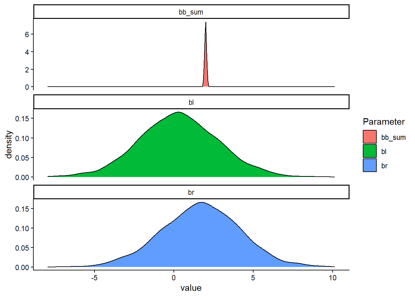
The model in this case is silly, we do not learn anything more from including the right leg after having the left leg in the model. The algorithm struggles because of the correlated parameter values and so, we have reached computational problems because of a bad model.
The posterior might still be the correct one. Let’s try to combine the parameter estimates (βLL and βRL) to see if their sum is what we are looking for.
Code
draws6.1 <- fit6.1$draws(format = "df")


p1 <- draws6.1 |>
  select(.iteration, bl, br) |>
  mutate(bb_sum = bl + br) |>
  pivot_longer(cols = bl:bb_sum,
               names_to = "Parameter") |>
  ggplot(aes(value, fill = Parameter)) + geom_density() +
  facet_wrap(~ Parameter, scales = "free_y", ncol = 1) +
  theme_classic()
Warning: Dropping 'draws_df' class as required metadata was removed.Code
p1