4  Drawing Directed Acyclic Graphs

Directed acyclic graphs (DAGs) are great for describing scientific models or systems that we might want to formally model using a statistical model. Using a DAG, we can describe assumptions regarding causal relationships among variables in our system. See (McElreath 2020, 128–28) for an introduction. Below are several examples of methods for drawing DAGs in R.

4.1 A basic DAG

4.1.1 Dagitty

Dagitty is an R package and a web interface for creating DAGs with additional functionality to identify variables to adjust to retrieve a causal effect given a specific graph. The web interface allows for point and click and the R package allows for creating graphs and finding adjustment sets programmatically.

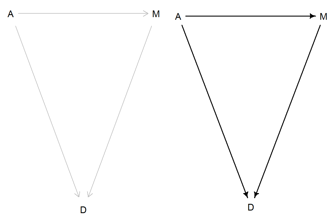
Below we are recreating DAG 5.1 (McElreath 2020, 129). The DAG has three variables, A, M and D. Using Dagitty we can define the basic graph by the associations between variables. The Dagitty package has a plot method for constructed graphs, adding coordinates makes it possible to control placement of variables in the plot. Using drawdag from the rethinking package makes the graph “fancier” (see ?rethinking::drawdag). Below both versions of DAG 5.1 are shown (Figure 4.1).

library(dagitty)
library(rethinking)

# Create the basic graph
dag5.1 <- dagitty( "dag{ A -> D; A -> M; M -> D }" )
# Define coordinates
coordinates(dag5.1) <- list( x=c(A=0,D=1,M=2) , y=c(A=0,D=1,M=0) ) 

# Display both graphs
par(mfrow = c(1,2))
plot(dag5.1); rethinking::drawdag(dag5.1)

Figure 4.1: DAG5.1 displayed using the Dagitty package and the rethinking package.

The arrows (edges) shows the (assumed) direction of the causal effect, variables (A, M and D; nodes).

4.2 ggdag: Using ggplot2 to draw DAGs

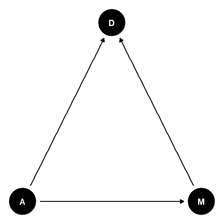
An alternative to the basic plotting functionality in dagitty and the alternative in the rethinking package is the the ggdag package that uses ggplot2in the background. This could be useful when we want to customize the plot. For now, we will simply recreate the above plots using ggdag.

library(ggdag)

ggdag(dag5.1) + theme_dag()

Figure 4.2: DAG5.1 displayed using the ggdag package

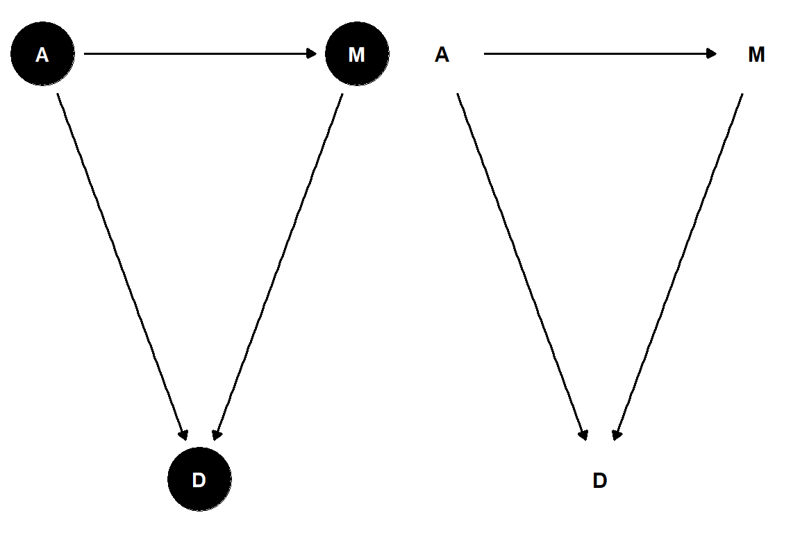
The ggdag package use the information on variable associations created with dagitty above to display the graph. We can take control over this process at multiple levels.

library(tidyverse)


dag_coords <-
  tibble(name = c("A", "M", "D"),
         x    = c(1, 3, 2),
         y    = c(2, 2, 1))


dag <-
  dagify(M ~ A,
         D ~ A,
         D ~ M,
         coords = dag_coords)


p1 <- dag |> 
  ggdag() + 
  theme_dag()



# Customizable plot 

p2 <- dag |>
  tidy_dagitty() |> 
  ggplot(aes(x = x, y = y, xend = xend, yend = yend)) +
  geom_dag_text(color = "black") +
  geom_dag_edges() + 
  theme_dag()



cowplot::plot_grid(p1, p2)

Figure 4.3: DAG5.1 displayed using the ggdag package, with customizations in the second panel

McElreath, Richard. 2020. Statistical Rethinking: A Bayesian Course with Examples in R and Stan. Second edition. Chapman & Hall/CRC Texts in Statistical Science Series. Boca Raton: CRC Press.