# Loading packages
library(cmdstanr)
library(rethinking)5 Chapter 4: Geocentric models
5.1 Stan
Stan is a probabilistic programming language that implements Hamiltonian Monte Carlo (HMC) sampling to approximate the joint probability distribution given a model and data (Carpenter et al. 2017). Stan serves as the back end for HMC inference in the rethinking, rstanarm, and brms R packages. Using Stan as a back end has the advantage of keeping all coding in a familiar environment. However, knowing how to build models directly in Stan provides greater control (McElreath 2020, 286–86). The purpose of these chapters is to become more familiar with Stan by fitting models from Statistical Rethinking directly in Stan.
Carpenter, Bob, Andrew Gelman, Matthew D. Hoffman, Daniel Lee, Ben Goodrich, Michael Betancourt, Marcus Brubaker, Jiqiang Guo, Peter Li, and Allen Riddell. 2017. “Stan : A Probabilistic Programming Language.” Journal of Statistical Software 76 (1). https://doi.org/10.18637/jss.v076.i01.
I will use cmdstanr as the R interface to Stan. This package allows us to define settings for the HMC sampler (or Stan’s optimization algorithm (Carpenter et al. 2017)) and retrieve HMC samples for use in R, post-sampling.
For reference, the Stan User’s guide and the Stan Reference Manual will be used when appropriate.
5.2 Model 4.1
The data used in m4.1 comes from Howell1 after filtering for ages >= 18.
data("Howell1")

d <- Howell1[ Howell1$age >= 18 , ]

str(d)
'data.frame': 352 obs. of 4 variables:
$ height: num 152 140 137 157 145 ...
$ weight: num 47.8 36.5 31.9 53 41.3 ...
$ age : num 63 63 65 41 51 35 32 27 19 54 ...
$ male : int 1 0 0 1 0 1 0 1 0 1 ...The model is defined as:
\[ \begin{align} h_i &\sim \operatorname{Normal}(\mu, \sigma) \\ \mu &\sim \text{Normal}(178, 20) \\ \sigma &\sim \operatorname{Uniform}(0, 50) \end{align} \]
data {
  int<lower=0> N;
  vector[N] h;
}
parameters {
  real mu;
  real<lower=0, upper=50> sigma;
}
model {
  mu ~ normal(178, 20);  // Prior for mu
  sigma ~ uniform(0,50); // Prior for sigma
  h ~ normal(mu, sigma); // likelihood
}
The symbol h refers to the list of heights, and the subscript i means each individual element of this list. It is conventional to use i because it stands for index. The index i takes on row numbers, and so in this example can take any value from 1 to 352 (the number of heights in d2$height). As such, the model above is saying that all the golem knows about each height measurement is defined by the same normal distribution, with mean μ and standard deviation σ. (McElreath 2020, 81).
The mathematical model definition contain the likelihood and priors for parameters μ and σ. To translate this model to Stan code we need three program blocks defined by their name and curly brackets (e.g., data { ...})1.
1 Stan has seven named programming blocks, all of which are optional but if they are part of a Stan program they must be specified in a specific order. The blocks are, in order, functions, data, transformed data, parameters, transformed parameters, model, and generated quantities. See Stan’s program blocks in the Reference manual.
Gelman, Andrew, and Jennifer Hill. 2007. Data Analysis Using Regression and Multilevel/Hierarchical Models. Analytical Methods for Social Research. Cambridge ; New York: Cambridge University Press.
In this model, the first block, data declares the data where N is the number of observation and h is a vector of heights with length N. The Reference Manual (Statistical Variable Taxonomy) indicates a difference between modeled and unmodeled data. According to (Gelman and Hill 2007, 367), modeled data are “data objects that are assigned probability distributions” while unmodeled data are not assigned distributions. In m4.1 we use the unmodeled data, N, to declare the size of the modeled data. The parameters block defines the parameters of interest, both μ (mu) and σ (sigma) are real numbers but a bound is placed on sigma corresponding to the uniform prior. The model block contains probability statements for the priors and the likelihood.
To compile the model we need to tell cmdstanr where the program file is located. I’ve collected all models in a sub folder in my project called models. A compiled model will be stored as an exe file in the same folder, if an up to date executable is present in the folder, the model will not be recompiled.
# Compiling the model
m4.1 <- cmdstan_model(stan_file = "models/m4-1.stan",
                      exe_file = "models/m4-1.exe")
Next, we need to prepare the data. Stan accepts a named list of variables. I’ll use dl (for data list) as a standard here. The data in this case is N, the number of observations, and h which are observed heights.
dl <- list(N = length(d$height),
           h = d$height)
To run the model we need to use cmdstanr again, this time with a command telling it to sample from the posterior. The model object is an R6 object2. We can access slots in the object using the $ operator. Slots can be functions (methods)3, like sample() which will perform HMC sampling, or check_syntax(), which will check the syntax in the Stan program.
2 See here for details.
3 See the cmdstanr documentation for methods and their arguments.
m4.1$check_syntax()Stan program is syntactically correctWe will run the sampler to get the posterior. We are saving the output from the sampler in fit4.1.
fit4.1 <- m4.1$sample(
        data = dl,                 # The list of variables
        iter_sampling = 2000,      # Number of iterations for sampling
        iter_warmup = 1000,        # Number of warm-up iterations
        chains = 1,                # Number of Markov chains
        refresh = 1000             # Number of iterations before each print
)
Running MCMC with 1 chain...
Chain 1 Iteration: 1 / 3000 [ 0%] (Warmup)
Chain 1 Iteration: 1000 / 3000 [ 33%] (Warmup)
Chain 1 Iteration: 1001 / 3000 [ 33%] (Sampling)
Chain 1 Iteration: 2000 / 3000 [ 66%] (Sampling)
Chain 1 Iteration: 3000 / 3000 [100%] (Sampling)
Chain 1 finished in 0.0 seconds.The object fit4.1 is another R6 object with several methods4. We can retreive the posterior draws from the model fit using the draws() method. We may want to extract the draws to summarize the posterior or perform predictions. Extracting the draws to a data frame makes it easy to work with the parameter values, however, other alternatives are possible. A list is recommended when models have a large number of parameters (see here).
4 See the here for the CmdStanMCMC object documentation.
draws <- fit4.1$draws(format = "df")The draws object created above can be used to create a figure similar to Figure 4.4 in (McElreath 2020, 86) (see Figure 5.1), together with marginal posteriors for the parameters in the model. I will use the tidyverse to wrangle and plot data in further examples.
library(tidyverse)
library(patchwork)

p1 <- draws |>
  ggplot(aes(mu, sigma)) +
  geom_point(alpha = 0.2,
             size = 3,
             color = "steelblue") +
  theme_classic()

p2 <- as_tibble(draws) |>
   pivot_longer(cols = c(mu, sigma)) |>
   ggplot(aes(value)) +
  geom_density() +
  facet_wrap(~ name,
             scales = "free") +
  theme_classic()


p1 / p2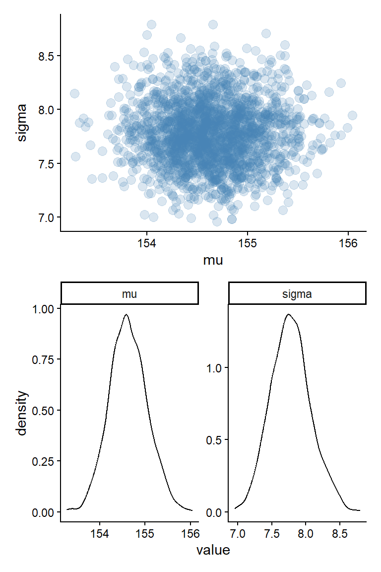
Summaries of the of the posterior are easily created from the draws data frame. To recreate quap output from (McElreath 2020, 88).
 as_tibble(draws) |>
   pivot_longer(cols = c(mu, sigma)) |>
  summarise(.by = name,
            m = mean(value),
            s = sd(value),
            lwr = quantile(value, 0.055),
            upr = quantile(value, 0.945))
# A tibble: 2 × 5
name m s lwr upr
<chr> <dbl> <dbl> <dbl> <dbl>
1 mu 155. 0.418 154. 155.
2 sigma 7.78 0.295 7.33 8.28The precis command also work on a fitted object.
precis(fit4.1) mean sd 5.5% 94.5% rhat ess_bulk
mu 154.632737 0.4179533 153.976793 155.328520 1.000349 1718.080
sigma 7.777691 0.2946020 7.325821 8.281121 1.001223 1856.8765.3 Model 4.2
In m4.2, the prior for μ is update to \(\mu \sim \operatorname{Normal}(178, 0.1)\), placing all of the information on the average of the prior.
data {
  int<lower=0> N;
  vector[N] h;
}
parameters {
  real mu;
  real<lower=0, upper=50> sigma;
}
model {
  mu ~ normal(178, 0.1);  // Prior for mu
  sigma ~ uniform(0,50); // Prior for sigma
  h ~ normal(mu, sigma); // likelihood
}
# Compiling the model
m4.2 <- cmdstan_model(stan_file = "models/m4-2.stan",
exe_file = "models/m4-2.exe")
fit4.2 <- m4.2$sample(
data = dl, # The list of variables
iter_sampling = 2000, # Number of iterations for sampling
iter_warmup = 1000, # Number of warm-up iterations
chains = 1, # Number of Markov chains
refresh = 1000 # Number of iterations before each print
)Running MCMC with 1 chain...
Chain 1 Iteration: 1 / 3000 [ 0%] (Warmup)
Chain 1 Iteration: 1000 / 3000 [ 33%] (Warmup)
Chain 1 Iteration: 1001 / 3000 [ 33%] (Sampling)
Chain 1 Iteration: 2000 / 3000 [ 66%] (Sampling)
Chain 1 Iteration: 3000 / 3000 [100%] (Sampling)
Chain 1 finished in 0.0 seconds.The model runs and results in a posterior that is heavily influenced by the prior on μ, for both parameters.
precis(fit4.2) mean sd 5.5% 94.5% rhat ess_bulk
mu 177.86235 0.09917671 177.70742 178.02641 1.001130 2081.397
sigma 24.58147 0.94860189 23.15512 26.22613 1.001695 1548.4215.4 Model 4.3 - Linear prediction
\[ \begin{align} h_i &\sim \operatorname{Normal}(\mu_i, \sigma) \\ \mu_i &= \alpha + \beta(x_i - \bar{x}) \\ \alpha &\sim \text{Normal}(178, 20) \\ \beta &\sim \text{Log-Normal}(0,1) \\ \sigma &\sim \operatorname{Uniform}(0, 50) \end{align} \]
/* Model 4.3 */
data {
  int<lower=0> N;  // Number of observations
  array[N] real h; // height data
  array[N] real w; // weight data
  real xbar;       // average height
}
parameters {
  real a;
  real<lower=0> b;
  real<lower=0, upper=50> sigma;
}
transformed parameters {
  array[N] real mu;
  for (i in 1:N) {
    mu[i] = a + b * (w[i] - xbar);
  }
}
model {
  a ~ normal(178, 20);
  b ~ lognormal(0,1);
  sigma ~ uniform(0,50);
  h ~ normal(mu, sigma);
}
To reflect the model definition, the code for Model 4.3 incorporates a transformed parameter, μ. This parameter is created from linear combination of two parameters α and β, and the predictor variable. Together they define deterministic formula for the mean in the normal distribution.
To run the model we need to add the weight data and an constant (xbar, \(\bar{x}\)), the average weight. Centering the predictor variable makes it possible to keep the prior from Model 4.1 for the intercept (α).
In the code below I’m preparing the data, compile the model and then fit it to data.
dl <- list(N = length(d$height),
           h = d$height,
           w = d$weight,
           xbar = mean(d$weight))


# Compiling the model
m4.3 <- cmdstan_model(stan_file = "models/m4-3.stan",
                      exe_file = "models/m4-3.exe")


fit4.3 <- m4.3$sample(
        data = dl,                 # The list of variables
        iter_sampling = 2000,      # Number of iterations for sampling
        iter_warmup = 1000,        # Number of warm-up iterations
        chains = 1,                # Number of Markov chains
        refresh = 1000             # Number of iterations before each print
)
Running MCMC with 1 chain...
Chain 1 Iteration: 1 / 3000 [ 0%] (Warmup)
Chain 1 Iteration: 1000 / 3000 [ 33%] (Warmup)
Chain 1 Iteration: 1001 / 3000 [ 33%] (Sampling)
Chain 1 Iteration: 2000 / 3000 [ 66%] (Sampling)
Chain 1 Iteration: 3000 / 3000 [100%] (Sampling)
Chain 1 finished in 0.6 seconds.precis(fit4.3)352 vector or matrix parameters hidden. Use depth=2 to show them. mean sd 5.5% 94.5% rhat ess_bulk
a 154.599725 0.26912303 154.1684111 155.0340998 1.000135 1939.863
b 0.904567 0.04352659 0.8350427 0.9751423 1.002990 1782.838
sigma 5.102773 0.18872204 4.8081206 5.4088172 1.000168 2175.8075.4.1 Plotting the posterior together with data
We can create a plot of the model implications using the parameters and a set of predictor values. In the code below I’m using weights from 20 to 70 to create a sequence of predictor values used by the model (w - xbar). Using expand_grid() makes it possible to do predictions over the whole range of the predictor variable (for each step in the constructed sequence). The data frame is summarized using the liner predictor formula (a + b * x, where x = w - xbar).
draws <- fit4.3$draws(format = "df")

draws |>
  select(a:sigma, .chain:.draw) |>
  expand_grid(
    data.frame(w = seq(from = 25, to = 70, by = 1))) |>
  mutate(x = w - dl$xbar) |>

  summarise(.by = c(x, w),
            mu = mean(a + b * x),
            lwr = quantile( a + b * x, 0.045),
            upr = quantile( a + b * x, 0.954)) |>

  ggplot(aes(w, mu)) +

  geom_point(data = d,
             aes(weight, height),
             color = "steelblue",
             shape = 21,
             size = 3) +

  geom_line() +
  geom_ribbon(aes(ymin = lwr,
                  ymax = upr),
              alpha = 0.2) +
  theme_classic()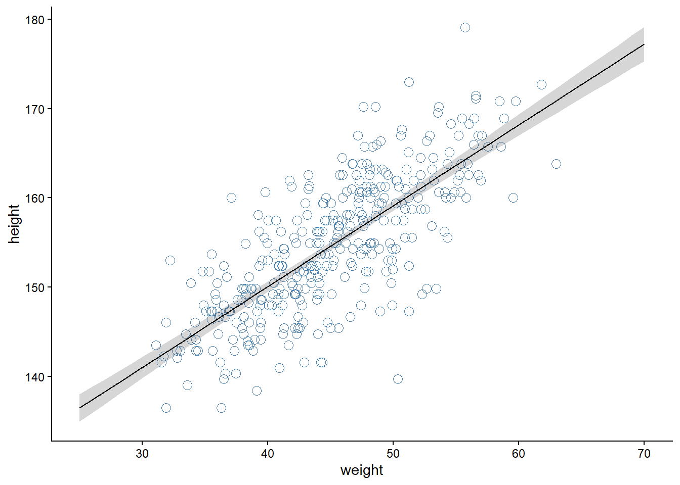
5.4.2 Extending the model to incorporate prior predictions
Model 4.3 is a fairly simple model, we can create a prior predictive check using a couple of lines in R (see (McElreath 2020, 95)). However, the model let’s construct a simple prior predictive check using Stan. We can do this by adding a prior_only flag together with an if-statement. We add the flag as data, if we want to sample only from the prior the flag is set to 1 and the likelihood is ignored.
\[ \begin{align} h_i &\sim \operatorname{Normal}(\mu, \sigma) \\ \mu &= \alpha + \beta(x_i - \bar{x}) \\ \alpha &\sim \text{Normal}(178, 20) \\ \beta &\sim \text{Log-Normal}(0,1) \\ \sigma &\sim \operatorname{Uniform}(0, 50) \end{align} \]
/* Model 4.3 */
data {
  int<lower=0> N;  // Number of observations
  array[N] real h; // height data
  array[N] real w; // weight data
  real xbar;       // average height
}
parameters {
  real a;
  real<lower=0> b;
  real<lower=0, upper=50> sigma;
}
transformed parameters {
  array[N] real mu;
  for (i in 1:N) {
    mu[i] = a + b * (w[i] - xbar);
  }
}
model {
  a ~ normal(178, 20);
  b ~ lognormal(0,1);
  sigma ~ uniform(0,50);
  h ~ normal(mu, sigma);
}
The below figure creates a prior predictive check similar to the one in Figure 4.5 (McElreath 2020, 95) Figure 5.3. We can use the same model to sample from the full posterior after setting the prior only flag to 0.
dl <- list(N = length(d$height),
           h = d$height,
           w = d$weight,
           xbar = mean(d$weight),
           prior_only = 1)


# Compiling the model
m4.3b <- cmdstan_model(stan_file = "models/m4-3b.stan",
                      exe_file = "models/m4-3b.exe")


fit4.3b_prior <- m4.3b$sample(
        data = dl,                 # The list of variables
        iter_sampling = 2000,      # Number of iterations for sampling
        iter_warmup = 1000,        # Number of warm-up iterations
        chains = 1,                # Number of Markov chains
        refresh = 1000             # Number of iterations before each print
)
Running MCMC with 1 chain...
Chain 1 Iteration: 1 / 3000 [ 0%] (Warmup)
Chain 1 Iteration: 1000 / 3000 [ 33%] (Warmup)
Chain 1 Iteration: 1001 / 3000 [ 33%] (Sampling)
Chain 1 Iteration: 2000 / 3000 [ 66%] (Sampling)
Chain 1 Iteration: 3000 / 3000 [100%] (Sampling)
Chain 1 finished in 0.6 seconds.draws <- fit4.3b_prior$draws(format = "df")
draws |>
slice_sample(n = 100) |>
select(a:b, .draw, .chain, .iteration) |>
expand_grid(data.frame(w = seq(from = 30, to = 70, by = 1))) |>
mutate(x = w - dl$xbar,
mu = a + b * x) |>
ggplot(aes(w, mu, group = .draw)) +
geom_line(alpha = 0.5) +
coord_cartesian(xlim = c(30, 70),
ylim = c(-100, 400)) +
geom_hline(yintercept = c(0, 272)) +
annotate("text",
x = c(30, 30),
y = c(-10, 282),
label = c("Embryo",
"World's tallest person (272 cm)"),
hjust = 0) +
theme_classic()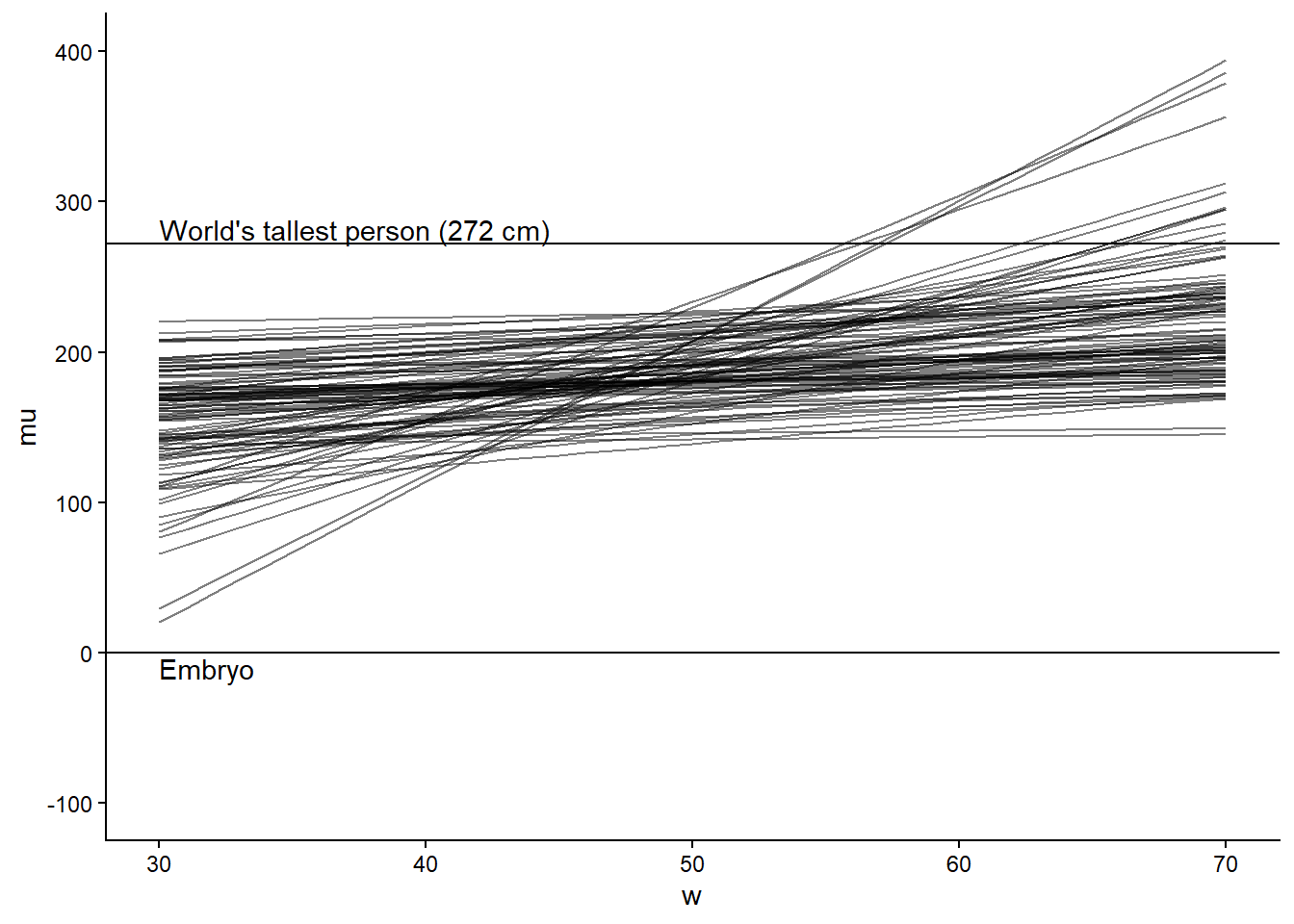
5.4.3 Prediction intervals from generated quantities
To build a prediction interval, similar to the one displayed in Figure 4.10 (McElreath 2020, 109), we can add a generated quantities block with a parameter y_pred that stores potential observations given the parameter values for α and β.
The formal model is the same as before, with the addition of a a new line indication predictions from the model. The predicted observations can also be used to generate posterior predictive checks (more on that in later chapters).
\[ \begin{align} h_i &\sim \operatorname{Normal}(\mu, \sigma) \\ \mu &= \alpha + \beta(x_i - \bar{x}) \\ \alpha &\sim \text{Normal}(178, 20) \\ \beta &\sim \text{Log-Normal}(0,1) \\ \sigma &\sim \operatorname{Uniform}(0, 50) \\ y^{\text{rep}}_i &\sim \text{Normal}(\mu_i, \sigma) \end{align} \]
/* Model 4.3 */
data {
  int<lower=0> N;  // Number of observations
  array[N] real h; // height data
  array[N] real w; // weight data
  real xbar;       // average height
}
parameters {
  real a;
  real<lower=0> b;
  real<lower=0, upper=50> sigma;
}
transformed parameters {
  array[N] real mu;
  for (i in 1:N) {
    mu[i] = a + b * (w[i] - xbar);
  }
}
model {
  a ~ normal(178, 20);
  b ~ lognormal(0,1);
  sigma ~ uniform(0,50);
  h ~ normal(mu, sigma);
}
Code
w_new <- seq(from = min(dl$w), to = max(dl$w), length.out = dl$N)
w_new <- dl$w

dl <- list(N = length(d$height),
           h = d$height,
           w = d$weight,
           xbar = mean(d$weight),
           N_new = length(w_new),
           w_new = w_new)


# Compiling the model
m4.3c <- cmdstan_model(stan_file = "models/m4-3c.stan",
                      exe_file = "models/m4-3c.exe")


fit4.3c <- m4.3c$sample(
        data = dl,                 # The list of variables
        iter_sampling = 4000,      # Number of iterations for sampling
        iter_warmup = 1000,        # Number of warm-up iterations
        chains = 1,                # Number of Markov chains
        refresh = 1000             # Number of iterations before each print
)
Running MCMC with 1 chain...
Chain 1 Iteration: 1 / 5000 [ 0%] (Warmup)
Chain 1 Iteration: 1000 / 5000 [ 20%] (Warmup)
Chain 1 Iteration: 1001 / 5000 [ 20%] (Sampling)
Chain 1 Iteration: 2000 / 5000 [ 40%] (Sampling)
Chain 1 Iteration: 3000 / 5000 [ 60%] (Sampling)
Chain 1 Iteration: 4000 / 5000 [ 80%] (Sampling)
Chain 1 Iteration: 5000 / 5000 [100%] (Sampling)
Chain 1 finished in 2.1 seconds.Code
draws <- fit4.3c$draws(format = "df")


# Extract the prediction interval
pred_int <- draws |>
  select(starts_with("y_pred")) |>
  pivot_longer(cols = everything()) |>
  mutate(name = as.numeric(gsub(".*?([0-9]+).*", "\\1", name))   ) |>
  inner_join(
    data.frame(name = 1:dl$N_new,
               w = dl$w_new)
    ) |>
  summarise(.by = c(w, name),
            mu = mean(value),
            lwr = quantile(value, 0.045),
            upr = quantile(value, 0.955))
Warning: Dropping 'draws_df' class as required metadata was removed.Joining with `by = join_by(name)`Code
draws |>
  select(a:sigma, .chain:.draw) |>
  expand_grid(
    data.frame(w = seq(from = min(dl$w), to = max(dl$w), by = 1))) |>
  mutate(x = w - dl$xbar) |>

  summarise(.by = c(x, w),
            mu = mean(a + b * x),
            lwr = quantile( a + b * x, 0.045),
            upr = quantile( a + b * x, 0.954)) |>

  ggplot(aes(w, mu)) +

  geom_point(data = d,
             aes(weight, height),
             color = "steelblue",
             shape = 21,
             size = 3) +

  geom_line() +
  geom_ribbon(aes(ymin = lwr,
                  ymax = upr),
              alpha = 0.2) +

    geom_ribbon(data = pred_int,
                aes(ymin = lwr,
                  ymax = upr),
              alpha = 0.2) +


  theme_classic()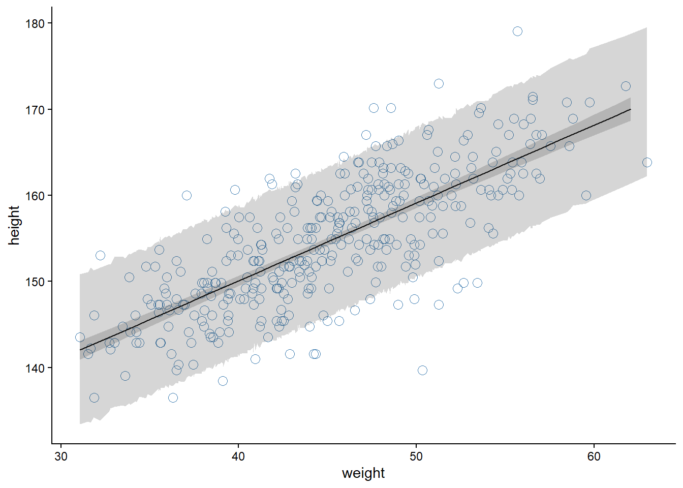
Code
draws |>
  slice_sample(n = 100) |>
  select(starts_with("y_pred"), .draw) |>

  pivot_longer(cols = starts_with("y_pred")) |>

  ggplot(aes(value, group = .draw)) +
  geom_density(color = "gray") +
  geom_density(data = d,
               aes(height, group = NULL),
               color = "steelblue",
               linewidth = 2) +

  theme_classic()
Warning: Dropping 'draws_df' class as required metadata was removed.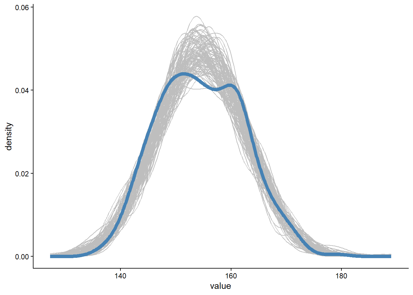
5.5 Model 4.5 - Curves from lines
Here we will use full Howell1 data set, which suggest a curved relationship between height and weight (Figure 5.6).
Code
d <- Howell1

d |>
  ggplot(aes(weight, height)) +
  geom_point(shape = 21,
             color = "steelblue",
             size = 3) +
  geom_smooth(se = FALSE) +
  theme_classic()
`geom_smooth()` using method = 'loess' and formula = 'y ~ x'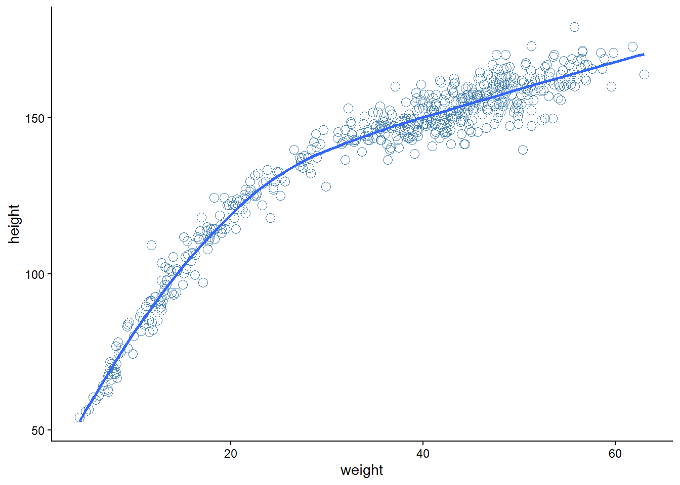
geom_smooth()
Model 4.5 is a parabolic model (rethink?). The predictor variables are constructed outside Stan by standardizing the weight variable and creating an extra squared variable.
x <- (d$weight - mean(d$weight)) / sd(d$weight)

dl <- list(h = d$height,
           x = x,
           x2 = x^2,
           N = length(d$height))
The model code (below) follows the definition, however, vectorization is used both in the likelihood and in the transformed parameters block (compared to e.g., m4.3).
\[ \begin{align} h_i &\sim \operatorname{Normal}(\mu_i, \sigma) \\ \mu &= \alpha + \beta_1x_i + \beta_2x^2_i \\ \alpha &\sim \text{Normal}(178, 20) \\ \beta_1 &\sim \text{Log-Normal}(0,1) \\ \beta_2 &\sim \text{Normal}(0,1) \\ \sigma &\sim \operatorname{Uniform}(0, 50) \\ \end{align} \]
/* Model 4.5 pp. 111
A parabolic model
*/
data {
  int<lower=0> N;
  vector[N] h;
  vector[N] x;
  vector[N] x2;
}
parameters {
  real a;
  real<lower=0> b1;
  real b2;
  real<lower=0, upper=50> sigma;
}
transformed parameters {
  vector[N] mu;
  // Vectorized transformed parameter
  mu = a + b1 * x + b2 * x2;

}
model {
  // Priors
  a ~ normal(178, 20);
  b1 ~ lognormal(0,1);
  b2 ~ normal(0,1);
  sigma ~ uniform(0,50);
  // Likelihood
  h ~ normal(mu, sigma);
}
# Compiling the model
m4.5 <- cmdstan_model(stan_file = "models/m4-5.stan",
exe_file = "models/m4-5.exe")
fit4.5 <- m4.5$sample(
data = dl, # The list of variables
iter_sampling = 2000, # Number of iterations for sampling
iter_warmup = 1000, # Number of warm-up iterations
chains = 1, # Number of Markov chains
refresh = 1000 # Number of iterations before each print
)Running MCMC with 1 chain...
Chain 1 Iteration: 1 / 3000 [ 0%] (Warmup)
Chain 1 Iteration: 1000 / 3000 [ 33%] (Warmup)
Chain 1 Iteration: 1001 / 3000 [ 33%] (Sampling)
Chain 1 Iteration: 2000 / 3000 [ 66%] (Sampling)
Chain 1 Iteration: 3000 / 3000 [100%] (Sampling)
Chain 1 finished in 1.2 seconds.precis(fit4.5)544 vector or matrix parameters hidden. Use depth=2 to show them. mean sd 5.5% 94.5% rhat ess_bulk
a 146.031481 0.3638369 145.454263 146.611950 1.001644 1063.2219
b1 21.740864 0.2954861 21.286581 22.214827 1.000685 1088.3467
b2 -7.785251 0.2687171 -8.213777 -7.358948 1.000994 965.6397
sigma 5.808603 0.1708473 5.544996 6.079611 1.000155 1673.1368Before recreating Figure 4.4 in the book we will fit the cubic regression model. The model formulation in the book differs from the quap code, below we follow the code formulation.
\[ \begin{align} h_i &\sim \operatorname{Normal}(\mu_i, \sigma) \\ \mu &= \alpha + \beta_1x_i + \beta_2x^2_i \\ \alpha &\sim \text{Normal}(178, 20) \\ \beta_1 &\sim \text{Log-Normal}(0,1) \\ \beta_2 &\sim \text{Normal}(0,10) \\ \beta_3 &\sim \text{Normal}(0,10) \\ \sigma &\sim \operatorname{Uniform}(0, 50) \\ \end{align} \]
/* Model 4.5 pp. 111
A cubic model
*/
data {
  int<lower=0> N;
  vector[N] h;
  vector[N] x;
  vector[N] x2;
  vector[N] x3;
}
parameters {
  real a;
  real<lower=0> b1;
  real b2;
  real b3;
  real<lower=0, upper=50> sigma;
}
transformed parameters {
  vector[N] mu;
  // Vectorized transformed parameter
  mu = a + b1 * x + b2 * x2 + b3 * x3;

}
model {
  // Priors
  a ~ normal(178, 20);
  b1 ~ lognormal(0,1);
  b2 ~ normal(0,10);
  b3 ~ normal(0,10);
  sigma ~ uniform(0,50);
  // Likelihood
  h ~ normal(mu, sigma);
}
# Adding the x3 variable to the data list
dl$x3 <- x^3
# Check that data (names) are in the list
names(dl)[1] "h" "x" "x2" "N" "x3"# Compiling the model
m4.6 <- cmdstan_model(stan_file = "models/m4-6.stan",
exe_file = "models/m4-6.exe")
fit4.6 <- m4.6$sample(
data = dl, # The list of variables
iter_sampling = 2000, # Number of iterations for sampling
iter_warmup = 1000, # Number of warm-up iterations
chains = 1, # Number of Markov chains
refresh = 1000 # Number of iterations before each print
)Running MCMC with 1 chain...
Chain 1 Iteration: 1 / 3000 [ 0%] (Warmup) Chain 1 Informational Message: The current Metropolis proposal is about to be rejected because of the following issue:Chain 1 Exception: normal_lpdf: Location parameter[1] is inf, but must be finite! (in 'C:/Users/706194/AppData/Local/Temp/RtmpCSfg58/model-19f83fab45cc.stan', line 32, column 2 to column 24)Chain 1 If this warning occurs sporadically, such as for highly constrained variable types like covariance matrices, then the sampler is fine,Chain 1 but if this warning occurs often then your model may be either severely ill-conditioned or misspecified.Chain 1 Chain 1 Iteration: 1000 / 3000 [ 33%] (Warmup)
Chain 1 Iteration: 1001 / 3000 [ 33%] (Sampling)
Chain 1 Iteration: 2000 / 3000 [ 66%] (Sampling)
Chain 1 Iteration: 3000 / 3000 [100%] (Sampling)
Chain 1 finished in 1.5 seconds.precis(fit4.6)544 vector or matrix parameters hidden. Use depth=2 to show them. mean sd 5.5% 94.5% rhat ess_bulk
a 146.751105 0.3148601 146.269130 147.267719 1.002276 1282.037
b1 14.994076 0.4856944 14.204386 15.793357 0.999951 1046.315
b2 -6.545119 0.2791786 -6.995778 -6.099924 1.000769 1112.067
b3 3.602562 0.2398135 3.224126 3.996971 1.001564 953.093
sigma 4.855248 0.1552362 4.619004 5.111007 1.001233 1588.362We will also re-run m4.3 with the complete data set after slight adjustment of the model to tackle the standardized weight variable (m4.3d).
/* Model 4.3 */
data {
  int<lower=0> N;  // Number of observations
  vector[N] h; // height data
  vector[N] x; // weight data
}
parameters {
  real a;
  real<lower=0> b;
  real<lower=0, upper=50> sigma;
}
transformed parameters {
  vector[N] mu;
  mu = a + b * x;
}
model {
  a ~ normal(178, 20);
  b ~ lognormal(0,1);
  sigma ~ uniform(0,50);
  h ~ normal(mu, sigma);
}m4.3d <- cmdstan_model(stan_file = "models/m4-3d.stan",
exe_file = "models/m4-3d.exe")
fit4.3d <- m4.3d$sample(
data = dl, # The list of variables
iter_sampling = 2000, # Number of iterations for sampling
iter_warmup = 1000, # Number of warm-up iterations
chains = 1, # Number of Markov chains
refresh = 1000 # Number of iterations before each print
)Running MCMC with 1 chain...
Chain 1 Iteration: 1 / 3000 [ 0%] (Warmup)
Chain 1 Iteration: 1000 / 3000 [ 33%] (Warmup)
Chain 1 Iteration: 1001 / 3000 [ 33%] (Sampling) Chain 1 Informational Message: The current Metropolis proposal is about to be rejected because of the following issue:Chain 1 Exception: normal_lpdf: Location parameter[1] is inf, but must be finite! (in 'C:/Users/706194/AppData/Local/Temp/Rtmp2lUtpo/model-4e303f763c81.stan', line 20, column 2 to column 24)Chain 1 If this warning occurs sporadically, such as for highly constrained variable types like covariance matrices, then the sampler is fine,Chain 1 but if this warning occurs often then your model may be either severely ill-conditioned or misspecified.Chain 1 Chain 1 Iteration: 2000 / 3000 [ 66%] (Sampling)
Chain 1 Iteration: 3000 / 3000 [100%] (Sampling)
Chain 1 finished in 0.8 seconds.precis(fit4.3d)544 vector or matrix parameters hidden. Use depth=2 to show them. mean sd 5.5% 94.5% rhat ess_bulk
a 138.292981 0.4049633 137.621139 138.929449 0.9999807 2374.089
b 25.953030 0.4135012 25.289961 26.602769 1.0004754 3123.811
sigma 9.390767 0.2904951 8.945647 9.867803 0.9996189 2788.711Prediction- and compatibility intervals are calculated from the models to reproduce Figure 4.11 (McElreath 2020, 112).
Code
# Prepare predictor variables for plotting
pred <- data.frame(x = seq(from = -2.5, to = 2, by = 0.1)) |>
  mutate(x2 = x^2,
         x3 = x^3)


draws4.3 <- fit4.3d$draws(format = "df")
draws4.5 <- fit4.5$draws(format = "df")
draws4.6 <- fit4.6$draws(format = "df")


# prob for intervals
lwr.prob <- 0.045
upr.prob <- 0.955


predictions <- bind_rows(
  draws4.3 |>
  select(a, b,sigma, .chain:.draw) |>
  expand_grid(pred) |>
  rowwise() |>
  mutate(y_rep = rnorm(1, a + b * x, sigma)) |>
  ungroup() |>
  summarise(.by = x,
            mu = mean(a + b * x),
            lwr = quantile(a + b * x, lwr.prob),
            upr = quantile(a + b * x, upr.prob),
            pred.lwr = quantile(y_rep, lwr.prob),
            pred.upr = quantile(y_rep, upr.prob))  |>
  mutate(type = "linear"),


  draws4.5 |>
  select(a:b2, sigma, .chain:.draw) |>
  expand_grid(pred) |>

  rowwise() |>
  mutate(y_rep = rnorm(1, a + b1 * x + b2 * x2, sigma)) |>
  ungroup() |>


  summarise(.by = x,
            mu = mean(a + b1 * x + b2 *x2 ),
            lwr = quantile(a + b1 * x + b2 *x2 , lwr.prob),
            upr = quantile(a + b1 * x + b2 *x2 , upr.prob),
            pred.lwr = quantile(y_rep, lwr.prob),
            pred.upr = quantile(y_rep, upr.prob)) |>
    mutate(type = "quadratic"),

  draws4.6 |>
  select(a:b3,sigma, .chain:.draw) |>
  expand_grid(pred) |>

  rowwise() |>
  mutate(y_rep = rnorm(1, a + b1 * x + b2 * x2 + b3 * x3, sigma)) |>
  ungroup() |>

  summarise(.by = x,
            mu = mean(a + b1 * x + b2*x2 + b3 * x3),
            lwr = quantile(a + b1 * x + b2*x2 + b3 * x3, lwr.prob),
            upr = quantile(a + b1 * x + b2*x2 + b3 * x3, upr.prob),
            pred.lwr = quantile(y_rep, lwr.prob),
            pred.upr = quantile(y_rep, upr.prob)) |>
    mutate(type = "cubic"))


# Fix the predictor variable for plotting
dplot <- d |>
  mutate(x = (weight - mean(weight)) / sd(weight) )

# Plot predictions
predictions |>
  mutate(type = factor(type, levels = c("linear", "quadratic", "cubic"))) |>
  ggplot(aes(x, mu)) +

  geom_line() +
  geom_ribbon(aes(ymin = lwr,
                  ymax = upr),
              alpha = 0.2) +

    geom_ribbon(aes(ymin = pred.lwr,
                  ymax =   pred.upr),
              alpha = 0.2) +

  # Add data
  geom_point(data = dplot,
             aes(x, height),
             shape = 21,
             color = "steelblue",
             size = 3,
             alpha = 0.5) +


  facet_wrap( ~ type, ncol = 3) +

  theme_classic() +
  theme(strip.background = element_rect(color = "white")) +
  labs(x = "Standardized weight",
       y = "Height")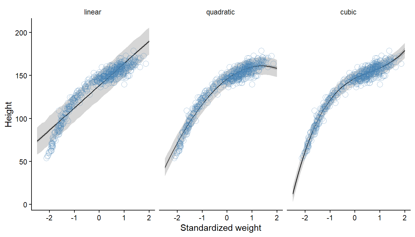
5.6 Model 4.7 - Splines
In the example with splines (Model 4.7), the rethinking::cherry_blossoms data are used. We filter the data directly to keep rows without NA in the doy variable.
data("cherry_blossoms")
d <- cherry_blossoms |>
  filter(complete.cases(doy))
Next we will create the synthetic predictor variables needed to run the model. I’m also preparing the first panel for Figure 4.13 in (McElreath 2020, 118).
library(splines)
num_knots <- 15
knot_list <- quantile(d$year,
                      probs = seq(0,1, length.out = num_knots))

B <- bs(d$year,
        knots = knot_list[-c(1, num_knots)],
        degree = 3,
        intercept = TRUE)

p1 <- data.frame(B) |>
  cbind(year = d$year) |>
  pivot_longer(starts_with("X")) |>
  ggplot(aes(year, value, group = name)) +
  geom_line() +
  theme_classic() +
  scale_y_continuous(breaks = c(0, 1)) +
  labs(x = "Year",
       y = "Basis value")
The model definition says that the outcome, D, is normally distributed with the parameters μ and σ. μ is a linear combination of an intercept (α) and a set of weights (wk) for each basis function (Bk). As noted on p. 118, the summation sign indicates that the products \(w_kB_{k,i}\) are all added together.
The Stan program is created without μ as part of transformed parameters, instead the a + w * B is entered directly in the likelihood. Stan uses * for matrix multiplication, B is a matrix with N rows and K columns and w is a vector of size K and the resulting products are summed to a vector of N, corresponding to the D outcome (see the Stan User’s Guide under Matrix notation and vectorization).
\[ \begin{align} D_i &\sim \operatorname{Normal}(\mu_i, \sigma) \\ \mu &= \alpha + \sum_{k=1}^K w_kB_{k,i} \\ \alpha &\sim \text{Normal}(100, 10) \\ w_k &\sim \text{Normal}(0,10) \\ \sigma &\sim \operatorname{Exponential}(1) \\ \end{align} \]
/* Model 4.7
A spline model of cherry blossoms
*/
data {
  int<lower=0> N; // N observations
  vector[N] D;    // outcome, day of blossom

  int<lower=0> K; // number of knots
  matrix[N,K] B;  // synthetic predictors
}
parameters {
  real a;               // intercept
  vector[K] w;          // weight parameters
  real<lower=0> sigma;  // sigma with lower bound
}
model {
  a ~ normal(100, 10);
  w ~ normal(0, 10);
  sigma ~ exponential(1);

  // Likelihood
  D ~ normal(a + B * w, sigma);

}
generated quantities {

  vector[N] y_pred = a + B * w;
  array[N] real y_rep = normal_rng(a + B * w, sigma);

}
The data needed for the Stan program is combined in a list. The Stan model is compiled, and executed.
dl <- list(N = nrow(d),
           D = d$doy,
           K = ncol(B),
           B = B)

m4.7 <- cmdstan_model(stan_file = "models/m4-7.stan",
                      exe_file = "models/m4-7.exe")

fit4.7 <- m4.7$sample(
        data = dl,                 # The list of variables
        iter_sampling = 2000,      # Number of iterations for sampling
        iter_warmup = 1000,        # Number of warm-up iterations
        chains = 1,                # Number of Markov chains
        refresh = 1000             # Number of iterations before each print
)
Running MCMC with 1 chain...
Chain 1 Iteration: 1 / 3000 [ 0%] (Warmup)
Chain 1 Iteration: 1000 / 3000 [ 33%] (Warmup)
Chain 1 Iteration: 1001 / 3000 [ 33%] (Sampling)
Chain 1 Iteration: 2000 / 3000 [ 66%] (Sampling)
Chain 1 Iteration: 3000 / 3000 [100%] (Sampling)
Chain 1 finished in 4.9 seconds.The model runs fine!
I’ve included two sets of generated quantities in the model definition y_pred and y_rep. y_pred is defined as the predicted value for each observations. Similar to what is done in (McElreath 2020, 119 (R code 4.78)), the observations are used to predict μ. y_rep are predictions using both μ and σ and can be used for posterior predictive checks (see also Gelman et al. 2014, ch. 6).
McElreath, Richard. 2020. Statistical Rethinking: A Bayesian Course with Examples in R and Stan. Second edition. Chapman & Hall/CRC Texts in Statistical Science Series. Boca Raton: CRC Press.
Gelman, Andrew, John B. Carlin, Hal Steven Stern, David B. Dunson, Aki Vehtari, and Donald B. Rubin. 2014. Bayesian Data Analysis. Third edition. Boca Raton: CRC Press.
Using estimates from the model we can prepare the last two panels of Figure 4.13 (McElreath 2020, 118).
draws <- fit4.7$draws(format = "df")


# Basis components times Weights

p2 <- data.frame(B) |>
  mutate(year = d$year) |>

  pivot_longer(cols = starts_with("X"),
               values_to = "B") |>

  inner_join(
    draws |>
  select(starts_with("w")) |>
  pivot_longer(cols = everything(), values_to = "w") |>
  mutate(name = gsub("\\]", "", gsub("w\\[", "X", name))) |>
  summarise(.by = name,
            w = mean(w))
  ) |>

  mutate(prod = B * w) |>

  ggplot(aes(year, prod, group = name)) +
  geom_line() +
  theme_classic() +
  labs(x = "Year",
       y = "basis * weigt")
Warning: Dropping 'draws_df' class as required metadata was removed.Joining with `by = join_by(name)`# mu
p3 <- draws |>
select(starts_with("y_pred")) |>
pivot_longer(cols = everything()) |>
inner_join(data.frame(name = paste0("y_pred[", 1:nrow(d), "]"),
year = d$year)) |>
summarise(.by = year,
mu = mean(value),
lwr = quantile(value, 0.015),
upr = quantile(value, 0.985)) |>
ggplot(aes(year, mu)) +
geom_point(data = d,
aes(year, doy),
alpha = 0.4,
color = "steelblue") +
geom_ribbon(aes(ymin = lwr,
ymax = upr),
alpha = 0.5) +
theme_classic() +
labs(x = "Year",
y = "Day in year")Warning: Dropping 'draws_df' class as required metadata was removed.Joining with `by = join_by(name)`p1 / p2 / p3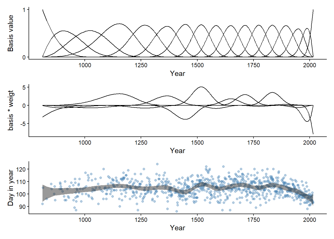
5.7 More on splines
As the weights are a “population” of parameters we could regularize them by having the model learn about the prior for \(w_k\) from the data. This introduces an hierarchical structure into the model. Extreme weights are regularized towards the global average of weights.
An alternative is to use a smoothing function that makes neighboring weights more similar, this is the penalized spline model described in Milad Kharratzadeh case study on Splines in Stand (found here)
Both the above alternatives are implemented in models 4.7b and 4.7c described below.
/* Model 4.7
A spline model of cherry blossoms including a hyperprior on the
weights parameters.
*/
data {
  int<lower=0> N; // N observations
  vector[N] D;    // outcome, day of blossom

  int<lower=0> K; // number of knots
  matrix[N,K] B;  // synthetic predictors
}
parameters {

  real a;               // intercept
  vector[K] w;          // weight parameters
  real<lower=0> wsigma; // hyperparameter on w
  real<lower=0> sigma;  // sigma with lower bound
}
model {
  a ~ normal(100, 10);
  w ~ normal(0, wsigma);
  wsigma ~ exponential(1);
  sigma ~ exponential(1);

  // Likelihood
  D ~ normal(a + B * w, sigma);

}
generated quantities {

  vector[N] y_pred = a + B * w;
  array[N] real y_rep = normal_rng(a + B * w, sigma);

}
/* Model 4.7
A spline model of cherry blossoms including a penalized spline
*/
data {
int<lower=0> N; // N observations
vector[N] D; // outcome, day of blossom
int<lower=0> K; // number of knots
matrix[N,K] B; // synthetic predictors
}
parameters {
real a; // intercept
vector[K] w; // weight parameters
real<lower=0> tau; // hyperparameter for smoothness
real<lower=0> sigma; // sigma with lower bound
}
transformed parameters {
vector[N] mu;
vector[K] wp;
wp[1] = w[1];
for (i in 2:K) {
wp[i] = wp[i-1] + w[i] * tau;
}
mu = a + B * wp;
}
model {
a ~ normal(100, 10);
w ~ normal(0, 1);
tau ~ exponential(0.2);
sigma ~ exponential(1);
// Likelihood
D ~ normal(mu, sigma);
}
generated quantities {
vector[N] y_pred = mu;
array[N] real y_rep = normal_rng(mu, sigma);
}Fitting both models shows the effect of the spline model on the wigglyness of the μ predictions.
Code
dl <- list(N = nrow(d),
           D = d$doy,
           K = ncol(B),
           B = B)

m4.7b <- cmdstan_model(stan_file = "models/m4-7b.stan",
                      exe_file = "models/m4-7b.exe")

fit4.7b <- m4.7b$sample(
        data = dl,                 # The list of variables
        iter_sampling = 2000,      # Number of iterations for sampling
        iter_warmup = 1000,        # Number of warm-up iterations
        chains = 1,                # Number of Markov chains
        refresh = 1000             # Number of iterations before each print
)
Running MCMC with 1 chain...
Chain 1 Iteration: 1 / 3000 [ 0%] (Warmup) Chain 1 Informational Message: The current Metropolis proposal is about to be rejected because of the following issue:Chain 1 Exception: normal_lpdf: Scale parameter is 0, but must be positive! (in 'C:/Users/706194/AppData/Local/Temp/Rtmps3H59y/model-1bb042bf4db9.stan', line 21, column 2 to column 24)Chain 1 If this warning occurs sporadically, such as for highly constrained variable types like covariance matrices, then the sampler is fine,Chain 1 but if this warning occurs often then your model may be either severely ill-conditioned or misspecified.Chain 1 Chain 1 Iteration: 1000 / 3000 [ 33%] (Warmup)
Chain 1 Iteration: 1001 / 3000 [ 33%] (Sampling)
Chain 1 Iteration: 2000 / 3000 [ 66%] (Sampling)
Chain 1 Iteration: 3000 / 3000 [100%] (Sampling)
Chain 1 finished in 3.8 seconds.Code
m4.7c <- cmdstan_model(stan_file = "models/m4-7c.stan",
                      exe_file = "models/m4-7c.exe")

fit4.7c <- m4.7c$sample(
        data = dl,                 # The list of variables
        iter_sampling = 2000,      # Number of iterations for sampling
        iter_warmup = 1000,        # Number of warm-up iterations
        chains = 1,                # Number of Markov chains
        refresh = 1000             # Number of iterations before each print
)
Running MCMC with 1 chain...
Chain 1 Iteration: 1 / 3000 [ 0%] (Warmup) Chain 1 Informational Message: The current Metropolis proposal is about to be rejected because of the following issue:Chain 1 Exception: normal_lpdf: Location parameter[1] is nan, but must be finite! (in 'C:/Users/706194/AppData/Local/Temp/Rtmps3H59y/model-1bb0481928a9.stan', line 44, column 2 to column 24)Chain 1 If this warning occurs sporadically, such as for highly constrained variable types like covariance matrices, then the sampler is fine,Chain 1 but if this warning occurs often then your model may be either severely ill-conditioned or misspecified.Chain 1 Chain 1 Informational Message: The current Metropolis proposal is about to be rejected because of the following issue:Chain 1 Exception: normal_lpdf: Location parameter[1] is nan, but must be finite! (in 'C:/Users/706194/AppData/Local/Temp/Rtmps3H59y/model-1bb0481928a9.stan', line 44, column 2 to column 24)Chain 1 If this warning occurs sporadically, such as for highly constrained variable types like covariance matrices, then the sampler is fine,Chain 1 but if this warning occurs often then your model may be either severely ill-conditioned or misspecified.Chain 1 Chain 1 Informational Message: The current Metropolis proposal is about to be rejected because of the following issue:Chain 1 Exception: normal_lpdf: Location parameter[1] is nan, but must be finite! (in 'C:/Users/706194/AppData/Local/Temp/Rtmps3H59y/model-1bb0481928a9.stan', line 44, column 2 to column 24)Chain 1 If this warning occurs sporadically, such as for highly constrained variable types like covariance matrices, then the sampler is fine,Chain 1 but if this warning occurs often then your model may be either severely ill-conditioned or misspecified.Chain 1 Chain 1 Informational Message: The current Metropolis proposal is about to be rejected because of the following issue:Chain 1 Exception: normal_lpdf: Location parameter[1] is nan, but must be finite! (in 'C:/Users/706194/AppData/Local/Temp/Rtmps3H59y/model-1bb0481928a9.stan', line 44, column 2 to column 24)Chain 1 If this warning occurs sporadically, such as for highly constrained variable types like covariance matrices, then the sampler is fine,Chain 1 but if this warning occurs often then your model may be either severely ill-conditioned or misspecified.Chain 1 Chain 1 Informational Message: The current Metropolis proposal is about to be rejected because of the following issue:Chain 1 Exception: normal_lpdf: Location parameter[1] is nan, but must be finite! (in 'C:/Users/706194/AppData/Local/Temp/Rtmps3H59y/model-1bb0481928a9.stan', line 44, column 2 to column 24)Chain 1 If this warning occurs sporadically, such as for highly constrained variable types like covariance matrices, then the sampler is fine,Chain 1 but if this warning occurs often then your model may be either severely ill-conditioned or misspecified.Chain 1 Chain 1 Informational Message: The current Metropolis proposal is about to be rejected because of the following issue:Chain 1 Exception: normal_lpdf: Location parameter[1] is nan, but must be finite! (in 'C:/Users/706194/AppData/Local/Temp/Rtmps3H59y/model-1bb0481928a9.stan', line 44, column 2 to column 24)Chain 1 If this warning occurs sporadically, such as for highly constrained variable types like covariance matrices, then the sampler is fine,Chain 1 but if this warning occurs often then your model may be either severely ill-conditioned or misspecified.Chain 1 Chain 1 Informational Message: The current Metropolis proposal is about to be rejected because of the following issue:Chain 1 Exception: normal_lpdf: Location parameter[1] is nan, but must be finite! (in 'C:/Users/706194/AppData/Local/Temp/Rtmps3H59y/model-1bb0481928a9.stan', line 44, column 2 to column 24)Chain 1 If this warning occurs sporadically, such as for highly constrained variable types like covariance matrices, then the sampler is fine,Chain 1 but if this warning occurs often then your model may be either severely ill-conditioned or misspecified.Chain 1 Chain 1 Informational Message: The current Metropolis proposal is about to be rejected because of the following issue:Chain 1 Exception: normal_lpdf: Location parameter[1] is nan, but must be finite! (in 'C:/Users/706194/AppData/Local/Temp/Rtmps3H59y/model-1bb0481928a9.stan', line 44, column 2 to column 24)Chain 1 If this warning occurs sporadically, such as for highly constrained variable types like covariance matrices, then the sampler is fine,Chain 1 but if this warning occurs often then your model may be either severely ill-conditioned or misspecified.Chain 1 Chain 1 Iteration: 1000 / 3000 [ 33%] (Warmup)
Chain 1 Iteration: 1001 / 3000 [ 33%] (Sampling)
Chain 1 Iteration: 2000 / 3000 [ 66%] (Sampling)
Chain 1 Iteration: 3000 / 3000 [100%] (Sampling)
Chain 1 finished in 10.6 seconds.Warning: 7 of 2000 (0.0%) transitions ended with a divergence.
See https://mc-stan.org/misc/warnings for details.Code
spline_plot <- function(draws, title, d) {

 p  <- draws |>
  select(starts_with("y_pred")) |>
  pivot_longer(cols = everything()) |>

  inner_join(data.frame(name = paste0("y_pred[", 1:nrow(d), "]"),
                        year = d$year)) |>


  summarise(.by = year,
            mu = mean(value),
            lwr = quantile(value, 0.015),
            upr = quantile(value, 0.985)) |>

  ggplot(aes(year, mu)) +

  geom_point(data = d,
             aes(year, doy),
             alpha = 0.4,
             color = "steelblue") +

  geom_ribbon(aes(ymin = lwr,
                  ymax = upr),
              alpha = 0.5)  +
  theme_classic() +
  labs(x = "Year",
       y = "Day in year",
       title = title)


}
Code
precis(fit4.7c) mean sd 5.5% 94.5% rhat ess_bulk
a 100.882397 2.4325752 96.956971 104.780601 1.0015640 1666.5075
tau 3.720255 1.1262894 2.199807 5.781576 0.9997009 559.2877
sigma 5.967107 0.1505125 5.726030 6.200651 0.9996995 2175.9398Code
draws_b <- fit4.7b$draws(format = "df")
draws_c <- fit4.7c$draws(format = "df")

p3 <- spline_plot(draws, title = "Spline model", d)
p3b <- spline_plot(draws_b, title = "Regularized weights", d)
p3c <- spline_plot(draws_c, title = "Locally regularized weights", d)


# Compare mean mu

post_mean <- function(draws, d, model ) {

  draws |>
  select(starts_with("y_pred")) |>
  pivot_longer(cols = everything()) |>

  inner_join(data.frame(name = paste0("y_pred[", 1:nrow(d), "]"),
                        year = d$year)) |>


  summarise(.by = year,
            mu = mean(value)) |>
    mutate(model = model)

}


p4 <- bind_rows(
  post_mean(draws, d, "m4.7"),
  post_mean(draws_b, d, "m4.7b"),
  post_mean(draws_c, d, "m4.7c"),
) |>
  ggplot(aes(year, mu, color = model)) +
  geom_line() +
  theme_classic() +
    labs(
      x = "Year",
       y = "Day in year",
      color = "Model")


p3 / p3b / p3c / p4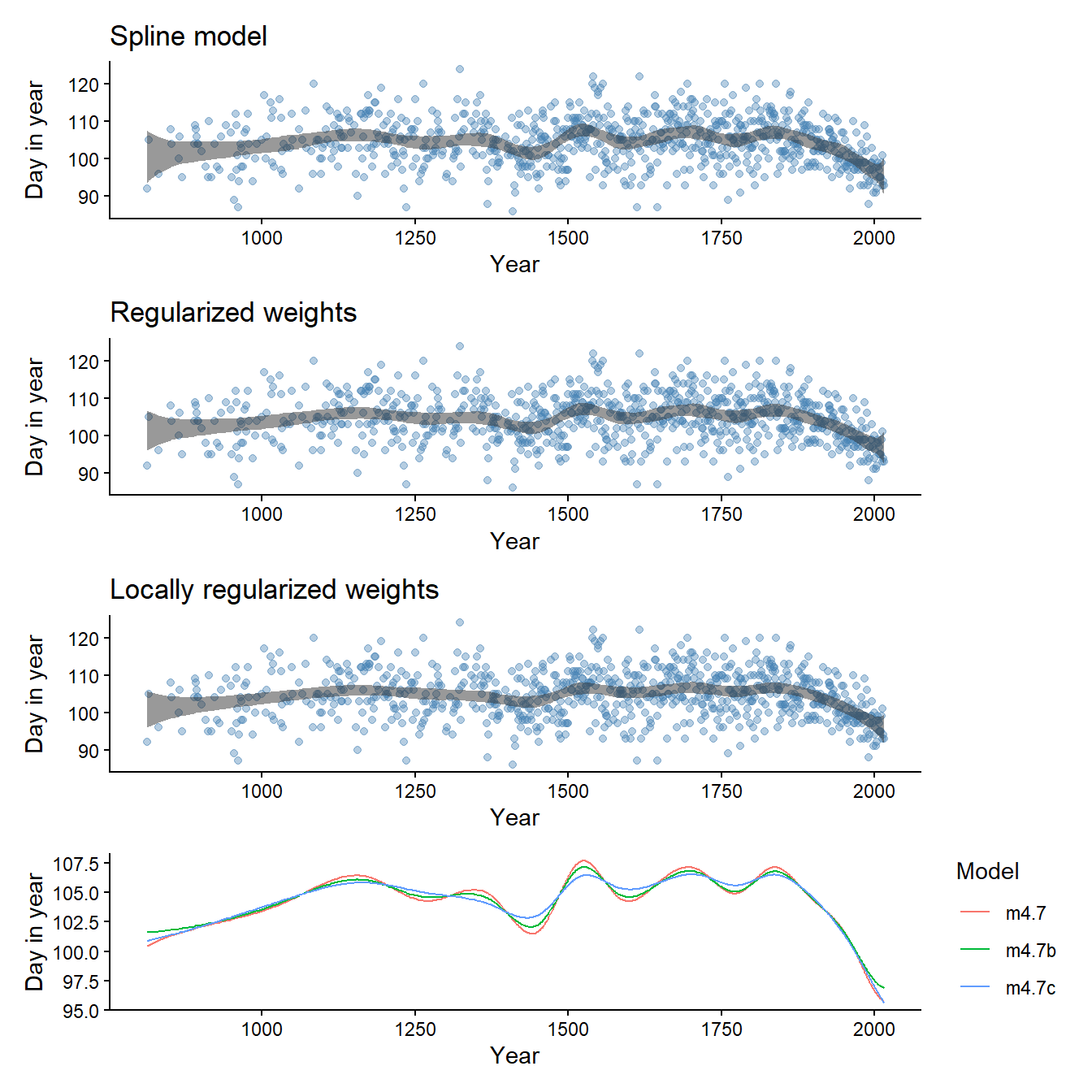
In later chapters we will discuss how to introduce hierarchical components and how to compare models for out of sample performance.