# Check if remotes is not installed, if TRUE, install remotes
if (!"remotes" %in% installed.packages()) install.packages(remotes)

# Check if exscidata is not installed, if TRUE, install exscidata from github
if (!"exscidata" %in% installed.packages()) remotes::install_github("dhammarstrom/exscidata")

# Load exscidata
library(exscidata)5 Creating figures
Data visualization is an efficient way to understand data. Using graphs, we can communicate characteristics of a data set in a way that would have been impossible with a limited number of summary statistics, such as the mean and standard deviation. In this sense, data visualization is a tool for exploratory and descriptive analysis. To use graphs for communicating data to others, additional layers of information are needed to provide context for graphical components. This requirement highlights the need for customization of data graphics for efficient communication. The tools we explore in this crash course offer an excellent environment for creating efficient, customized data visualizations. We will be able to develop standalone graphs based on data and incorporate them into reproducible reports with additional cross-referencing and descriptions.
The R ecosystem has several options for creating data visualizations. First, the base installation contains several functions for creating graphics. Additionally, lattice (see e.g. here) and tinyplot provide user-friendly extensions of the base R functionality, and tidyplot was introduced to provide a simple syntax for creating figures. However, in this course, we will focus on ggplot2 because it is powerful, well-documented, and widely used.
5.1 Loading data for our examples
To follow along in the examples below you will need some data. In this chapter we will work with the millward data set that is a part of the exscidata package. To install the package (exscidata) you will need another package, called remotes.
The code below first checks if the package remotes is installed, or more specifically, if "remotes" cannot be found in the list of installed packages. Using the if function makes install.packages(remotes) conditional. If we do not find "remotes" among installed packages, then install remotes.
The next line of code does the same with the exscidata package. However, since the package is not on CRAN but hosted on GitHub we will need to use remotes to install it. The part of the second line of code that says remotes::install_github("dhammarstrom/exscidata") uses the function install_github without loading the remotes package. The last line of the code below loads the package exscidata using the library function.
Next we need to load the tidyverse package. This package in turn loads several packages that we will use when transforming data and making our figures. I will include the line of code that checks if the package is installed, if not, R will download and install it. We subsequently load the package using library.
# Check if tidyverse is not installed, if TRUE, install remotes
if (!"tidyverse" %in% installed.packages()) install.packages(tidyverse)

library(tidyverse)
To follow along in this chapter you may want to start up a new Quarto file (.qmd), and store this file in your working directory. In this file you can add code to incrementally create figures and store commands used for loading packages. You will most likely work interactively with your first graphs, this means that you will go back and forth between different sections in your quarto-file and execute different to see intermediate results. Remember that you need to execute code in a specific sequence to create a graph, this means you should also structure your code in that way.
We are now ready to explore the data set. But first we should talk about the main components of the ggplot2 system.
5.2 The main components of the ggplot2 system
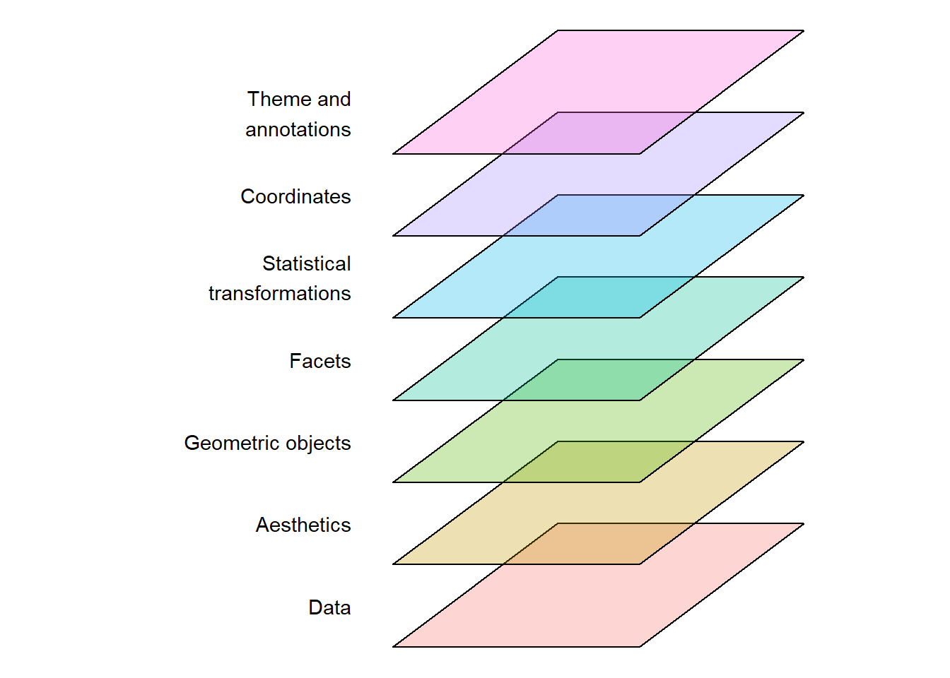
The ggplot2 system makes it possible to create a wide variety of data visualusations using a standard “grammar of graphics”. A graph is constructed using multiple layers of components (Figure 5.1) where mapping of data to different geometric objects and a coordinate system creates the visualization. When using the ggplot2 system we can think of the resulting graph as containing data that has been mapped to different shapes, colors, sizes, and coordinates, all of which determine what is being visualized.
When we map data in ggplot we use a specific function, aes() (short for aesthetic). We will use this inside the main engine, ggplot(). For this first simple example, we will create a data set by simulating some data1.
1 When you simulate data in R, you can tell R what should be the starting point in the random number generator. Using set.seed(100), we can recreate the same numbers from our “number generator” later.
In the example below, we use rnorm() to simulate numbers from a normal distribution. Using the arguments n = 10, mean = 0, and sd = 1, we simulate the process of randomly picking ten numbers from a distribution with a mean of 0 and a standard deviation of 1. These numbers are stored in a data frame that is assigned to an object that we have named d.
# Set the seed for random generation of numbers
set.seed(100)

# Store data in a data frame
d <- data.frame(Xdata = rnorm(10, mean = 0, sd = 1),
                  Ydata = rnorm(10, mean = 10, sd = 2))
The data set consists of two variables, we call them Xdata and Ydata. We will start the process of creating the graph by creating the canvas, and this basically sets the border of the figure we want to create. The ggplot() function takes the data set as its first argument, followed by the aes() function that maps data to coordinates and other attributes. In this case, we have mapped our data to the x- and y-coordinates of the figure.
ggplot(data = d, aes(x = Xdata, y = Ydata))ggplot canvas.
As you can see in Figure 5.2, the code above creates an “empty canvas” that has enough room to visualize our data. The x- and y-axes are adjusted to give room for graphical representations of the data. Next we need to add geometric shapes (geom for short). These are functions that we add to the plot using the + sign. These functions all start with geom_ and has and ending that describes the geometric shape, like for example point or line.
We will add geom_point() to our empty canvas as plotted in Figure 5.2. The geom_point function inherits the mapping from from ggplot(). Shapes, in this case points will be placed according to x- and y-coordinates specified in aes() used in the main ggplot function call. This means that we do not need to specify anything in geom_point at this stage.
ggplot(d, aes(x = Xdata, y = Ydata)) + geom_point()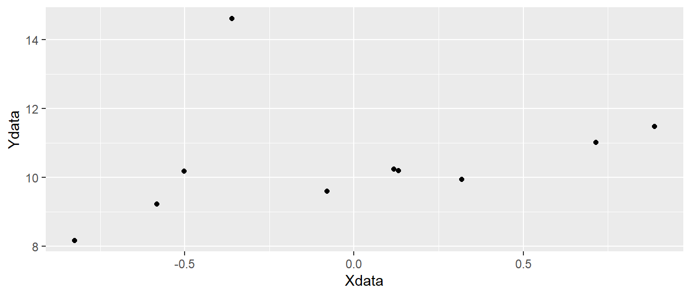
ggplot canvas with points added.
In Figure 5.3 we have added black points to each pair of observations in our data set representing x and y coordinates.
To extend the example we will add data to our data set. In the code below, we create a new variable in the data set using $ effectively giving us a new column in the data. We use rep("A", 5) to replicate the letter A five times and the same for B. The c() function combines the two in a single vector. We can use head(dat) to see what we accomplished with these operations. The head() function prints the first six rows from the data set.
d$z <- c(rep("A", 5), rep("B", 5))

head(d)
Xdata Ydata z
1 -0.50219235 10.179772 A
2 0.13153117 10.192549 A
3 -0.07891709 9.596732 A
4 0.88678481 11.479681 A
5 0.11697127 10.246759 A
6 0.31863009 9.941367 BWe can see that we have an additional variable, z that contains the letters "A" and "B". This new variable can be used to add more information to the plot. Let’s say that we want to map the z variable to different colors. We do this by adding color = z to aes. This means that we want the z variable to determine colors.
ggplot(d, aes(x = Xdata, y = Ydata, color = z)) + geom_point()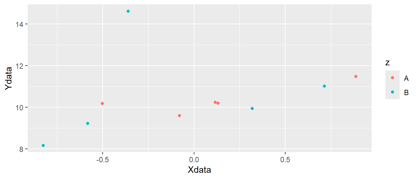
ggplot canvas with colored points added.
In Figure 5.4 we can see that different colors are used for the two letters "A" and "B". Other attributes can also be specified like shape, fill or size. The shape specifies the appearance of the points. When we use use data to map to shapes, ggplot2 will start from the standard set of shapes available in R, as displayed in Figure 5.5.
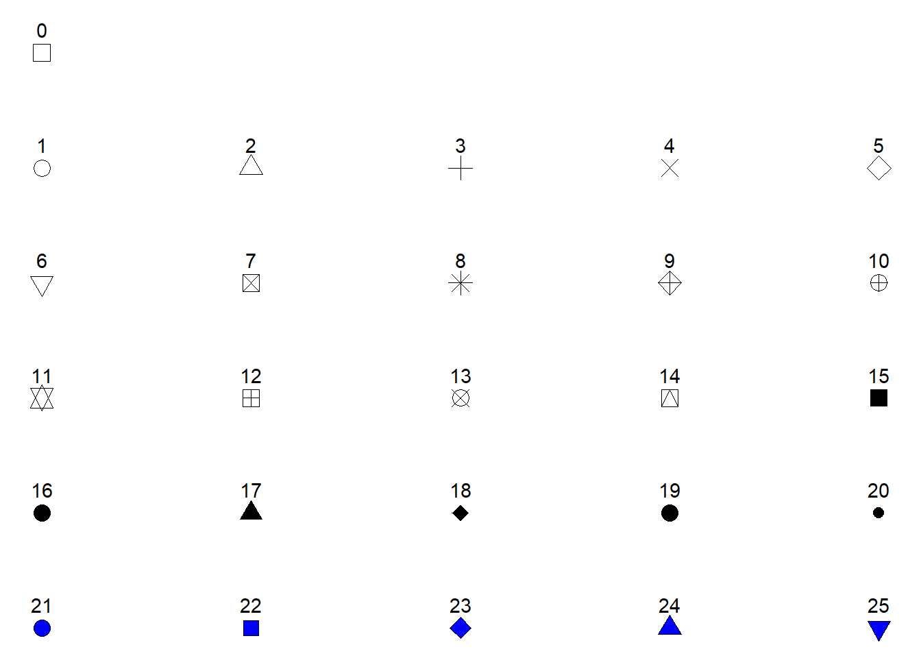
Shapes 0 to 25 can change colors while shapes 21 to 25 may have different border colors but also different fill colors. We may use this information to change the shape, color and fill of our points. Let’s say that instead of colored points we want filled points. We would then change the color = z argument to fill = z and select a point shape that can be filled (shapes 21-25, see Figure 5.5). Notice in the code below that shape = 21 has been added to geom_point(). We have specified how points should be displayed.
ggplot(d, aes(x = Xdata, y = Ydata, fill = z)) + geom_point(shape = 21)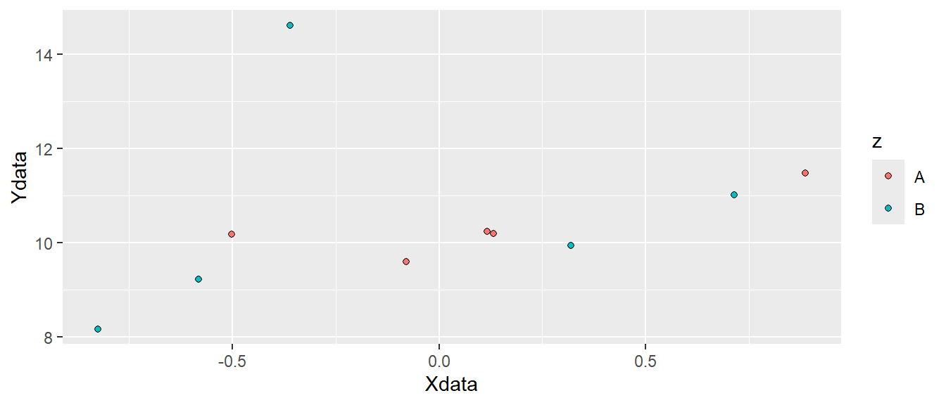
ggplot canvas with filled points added.
Since shape is an attribute we can map data to it. If we want data to determine both shape and fill we could add this information in the aes() function by setting both shape = z and fill = z. We now have to specify what shapes ggplot should use in order to be sure we can combine both shapes and fill. We will use scale_fill_manual and scale_shape_manual to do this. These functions lets you specify different values for aesthetics. Notice that we removed shape = 21 from the geom_point() function, but we added size to increase the size of the points (see Figure 5.7).
ggplot(d, aes(x = Xdata, y = Ydata, fill = z, shape = z)) +
  geom_point(size = 3) +
  scale_fill_manual(values = c("red", "green")) +
  scale_shape_manual(values = c(21, 23))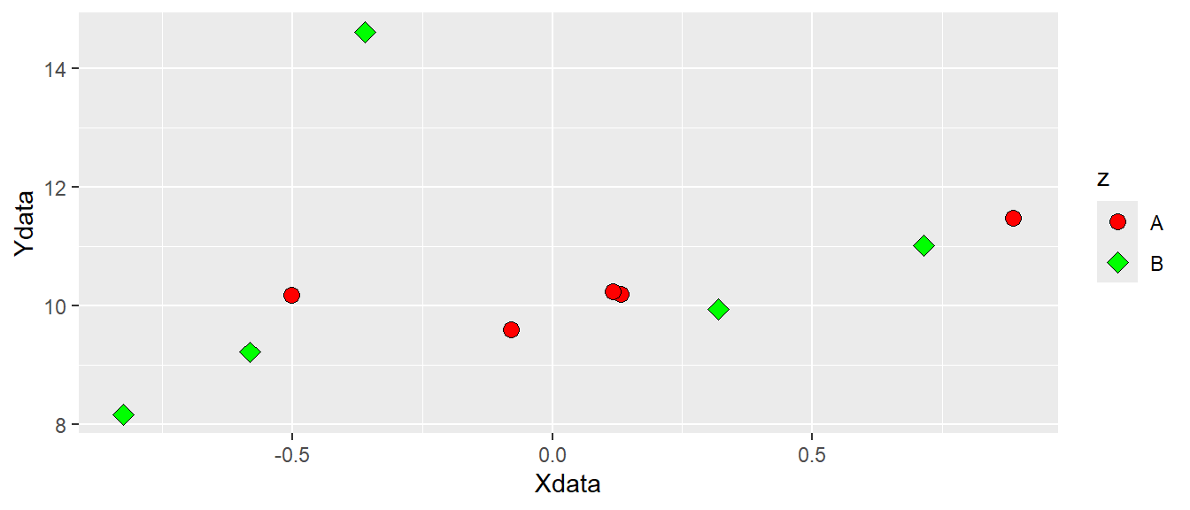
5.3 Different geoms using real data
We have seen that the basic ggplot2 figure maps underlying data to coordinates and geometric representations, such as points. We will go further by using some real data. We will be using the millward data set from the exscidata-package. We will start by loading the data and select a few columns that we are interested in.
By using data("millward") we will load the data set that is part of the exscidata-package to our environment. By looking at the environment tab you can see that this operation adds a data set to the environment. It has 52 observations and 3 variables. Using the glimpse() function from dplyr (which is loaded by loading tidyverse) we will get an overview of all variables in the data set. I have omitted the output from the code below, feel free to run the code on your own.
By typing ?millward in your R console you will open up a description of the data set. The three variables in the data set describes measures of total ribonucleic acid (RNA) and protein synthesis in skeletal muscle of two groups of rats. Group A represent animals given a control diet and B represent animals that are starved or given a protein-free diet.
# Load the data and have a first look
data("millward")
glimpse(millward)
5.3.1 One-dimensional visualizations
To get a sense of the distribution of a continous variable we might use visualizations that convey information on where we find our observations along a single axis. This can be done using a density plot, a histogram or a dotplot (although more alternatives are possible).
ggplot(data = millward, aes(x = protein_synthesis)) + geom_density()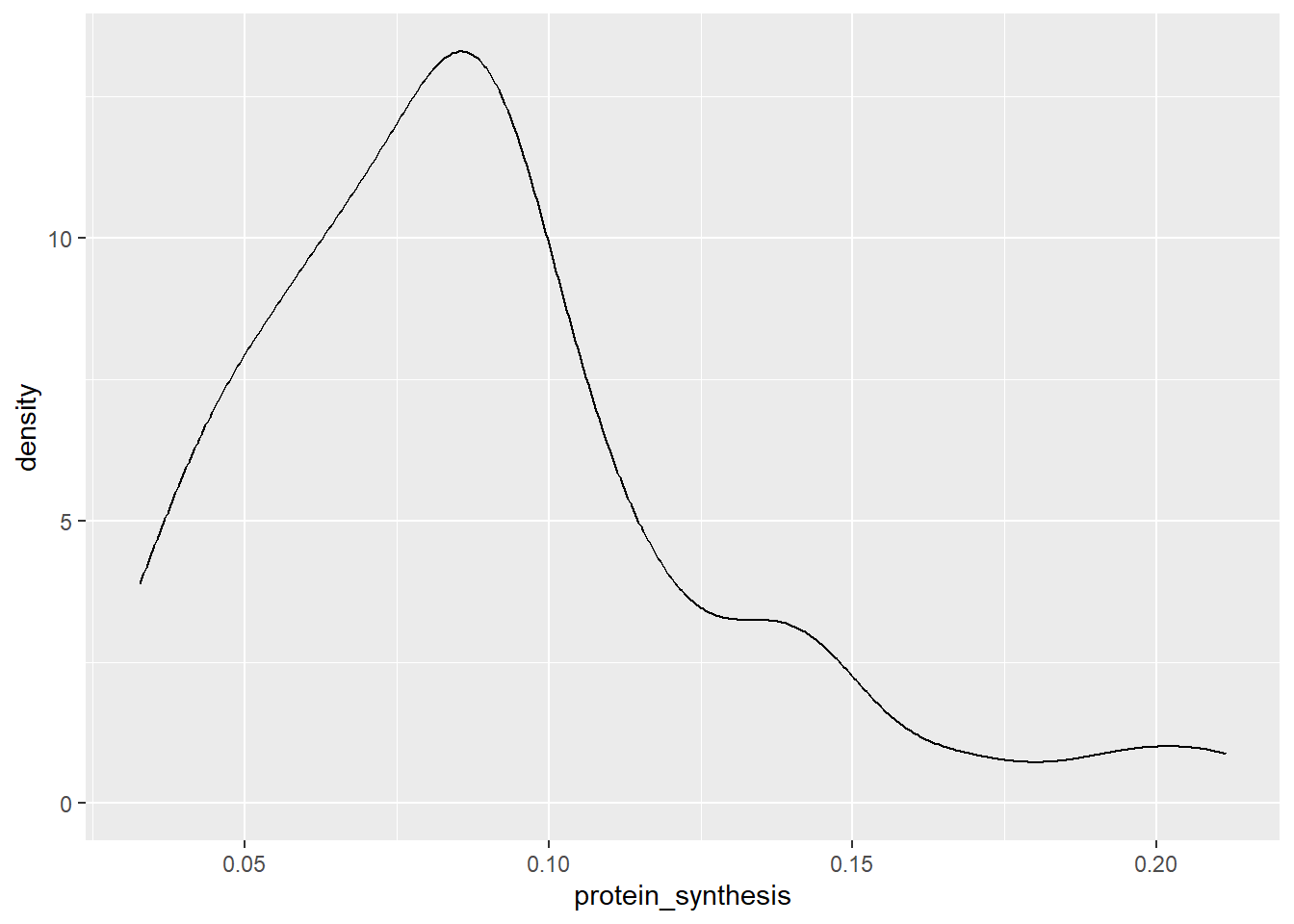
In this case, a density plot puts our variable of interest on the x-axis and calculates a weighted average of the number of observeations. The density plot above is basically a smoothed version of a histogram. In a histogram the height of each bar represent the count in each bin. Sometimes the binwidth can be manually changed.
ggplot(data = millward, aes(x = protein_synthesis)) + geom_histogram(binwidth = 0.01)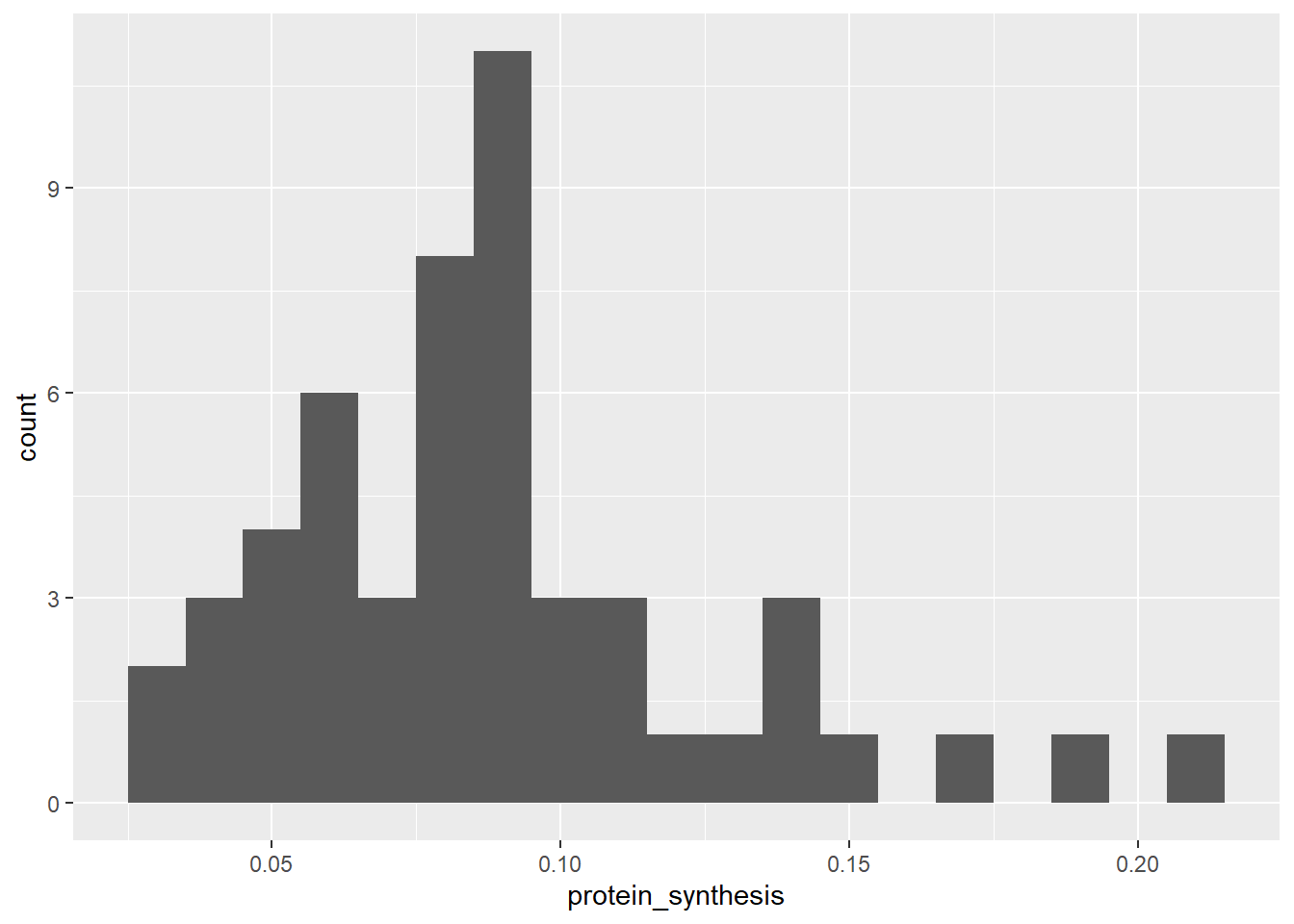
Another variation of the same basic idea (number of observations along a continous measurement), is the dotplot. In this variation each dot represent an observation that belongs to a bin.
ggplot(data = millward, aes(x = protein_synthesis)) + geom_dotplot(binwidth = 0.01)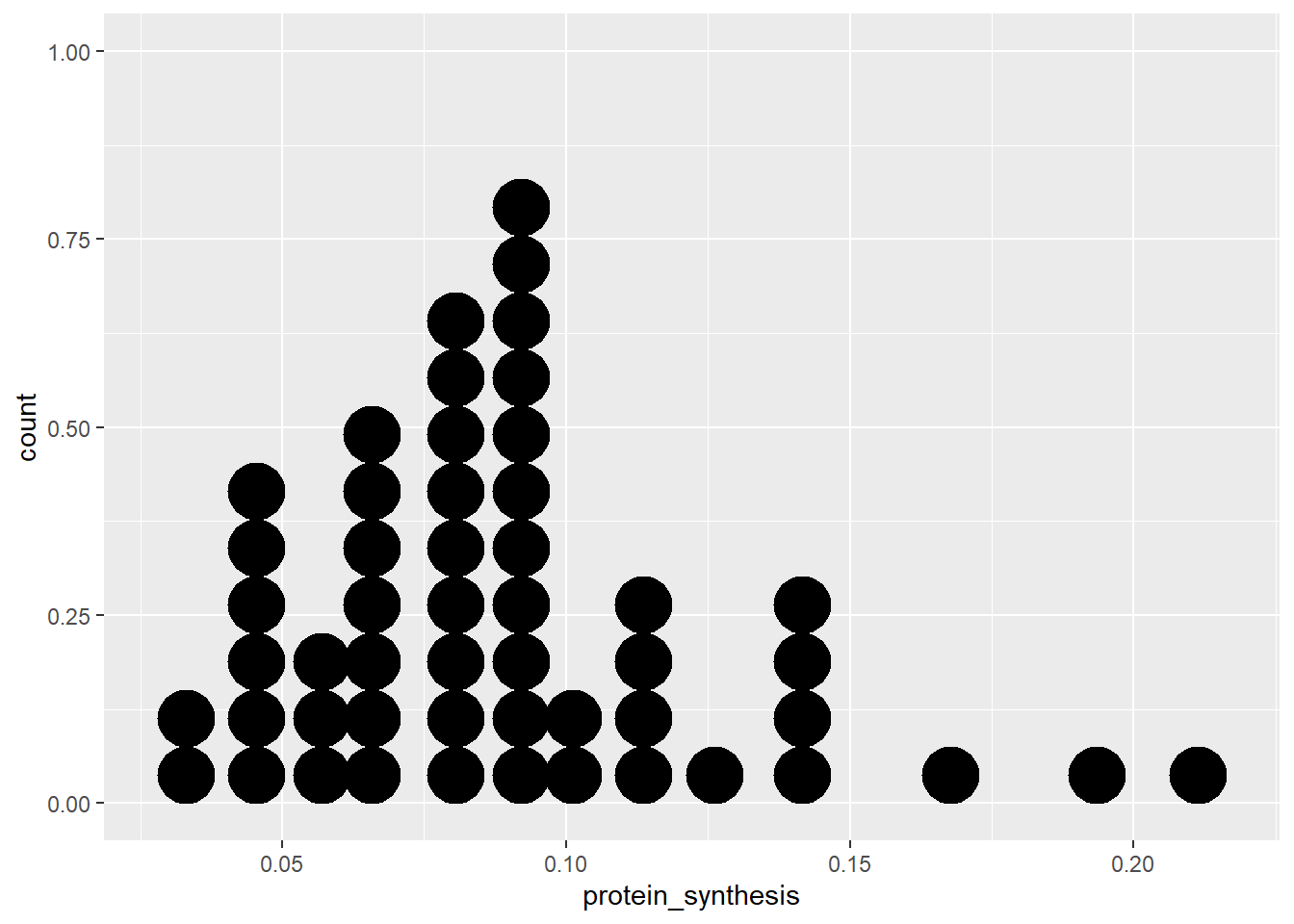
When the variable we want to display isn’t continuous, a bar plot could be used to display the number of observations per category. Instead of visualizing the continuous variable protein_synthesis, let’s try the group variable.
ggplot(data = millward, aes(x = group)) + geom_bar()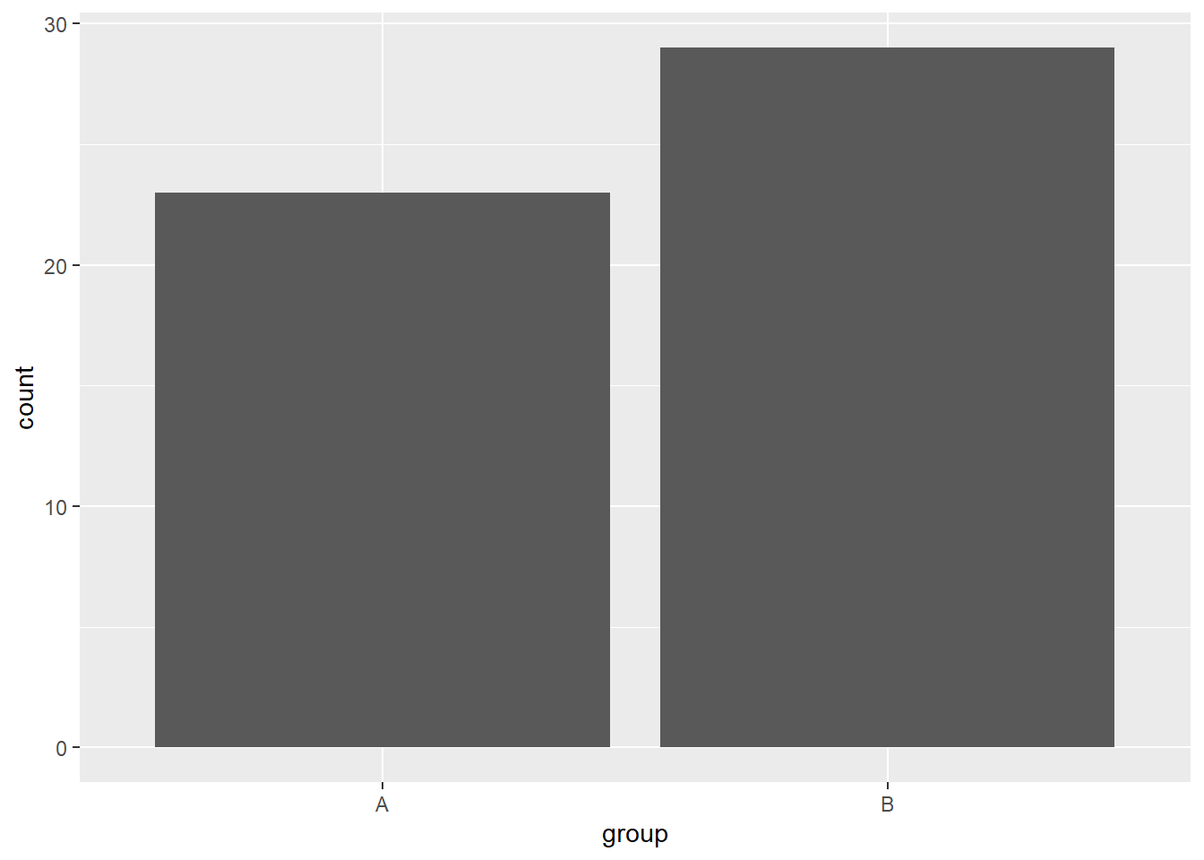
As we can see from the above examples, ggplot2 has many built in geometric representations capable of quickly displaying underlying data. All of the above examples includes data transformation of the y-axis to produce the graphs. This makes it considerably easier to produce effective visualizations.
The use of ready-made geoms with many sensible default settings extends to two-dimensional figures.
5.3.2 Two-dimensional visualizations
Two continous variables can be plotted using a scatterplot, this can be accomplished in ggplot2 using geom_point. Let’s see how RNA abundance relate to protein synthesis.
ggplot(data = millward, aes(x = RNA, y = protein_synthesis)) + geom_point()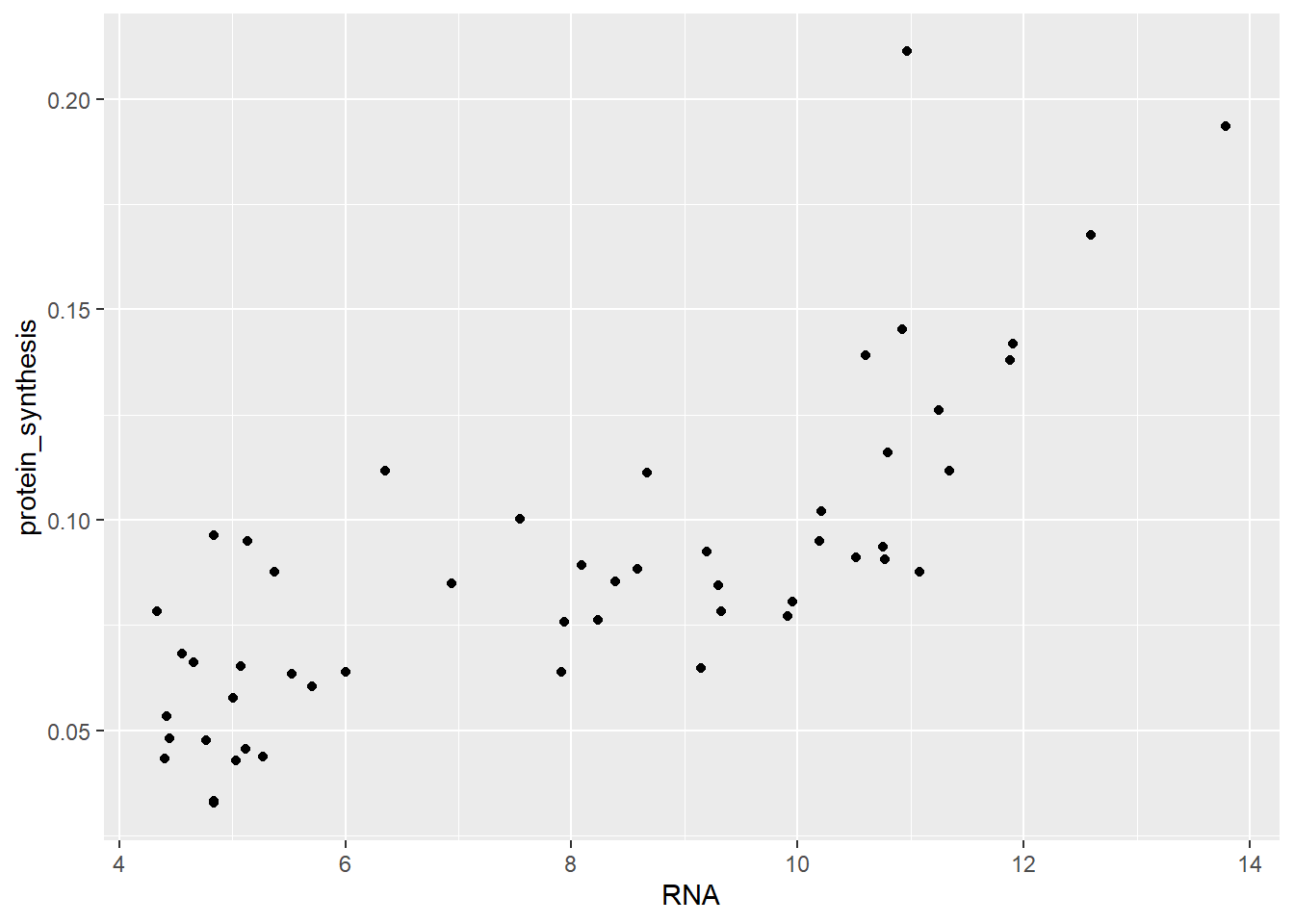
Notice that we specify x- and y-axis aesthetics inside aes above. As we will see in subsequent plots, we do not need to specify x- and y-axis, they can be implicitly specified by their positions in the aes function.
Similarly to a one-dimensional display of the distribution of observations along an axis we can use a two-dimensional density plot of show the relative concentration of observations.
ggplot(data = millward, aes(RNA, protein_synthesis)) + geom_density_2d()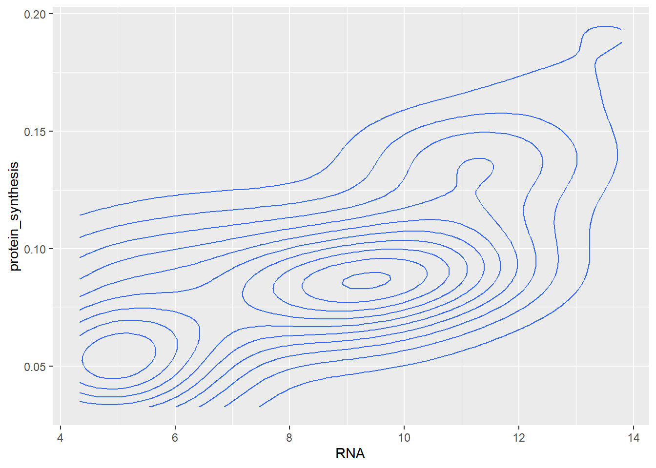
The two-dimensional density plot transforms the data in the visualisation step, similarly, smoothed trend to the plot requires transformation of the data. Using geom_smooth, ggplot2 will calculate required statistics to display, e.g. a linear trend in the data.
ggplot(data = millward, aes(RNA, protein_synthesis)) + geom_smooth(method = "lm")`geom_smooth()` using formula = 'y ~ x'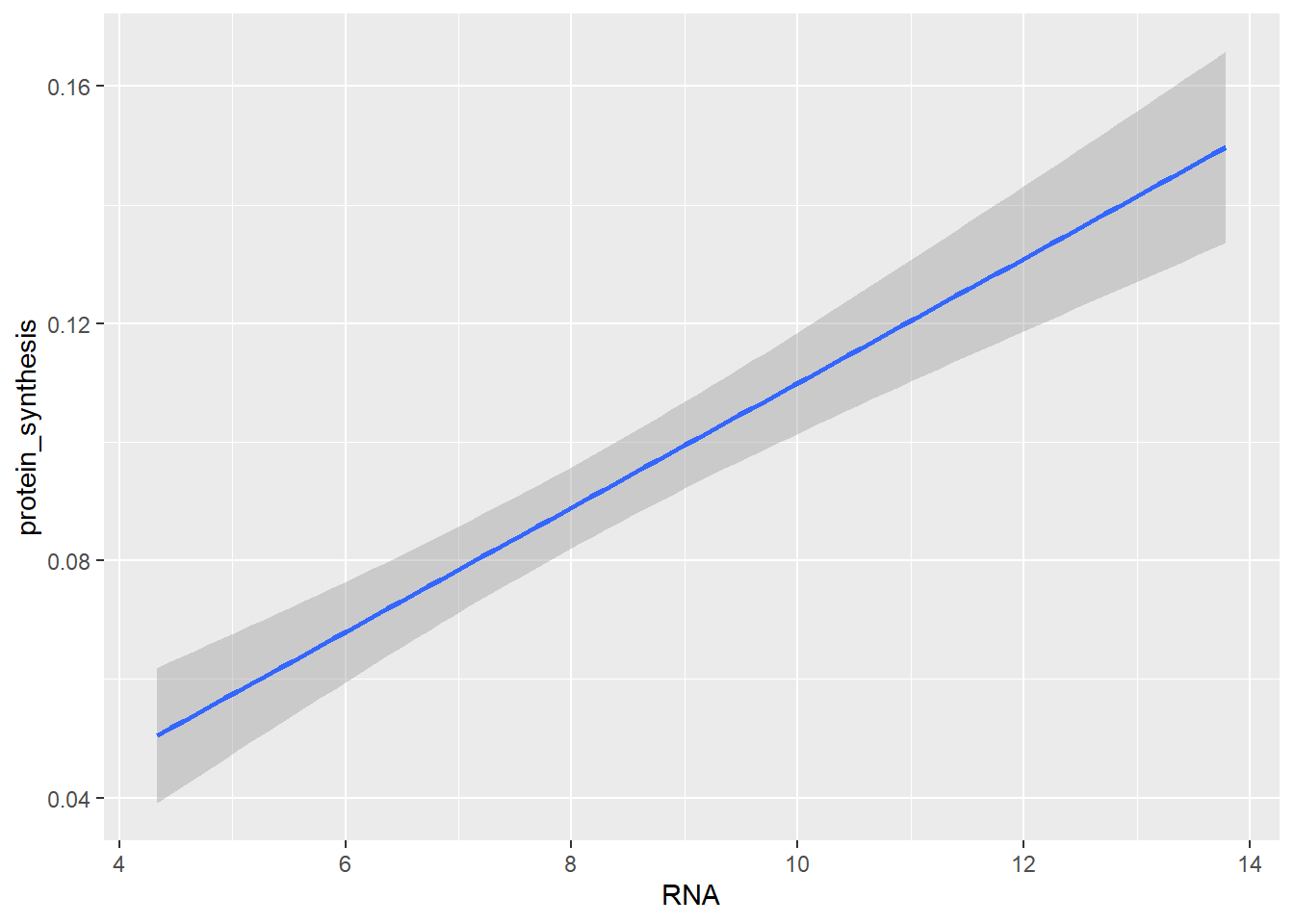
Notice the use of method = "lm" in the geom_smooth layer. This is an example of geom-specific setting that is needed to tweek the graph.
Using the ggplot2syntax we can of course combine all the above figures into one graph.
ggplot(data = millward, aes(RNA, protein_synthesis)) +
  geom_point() +
  geom_density_2d() +
  geom_smooth(method = "lm")
`geom_smooth()` using formula = 'y ~ x'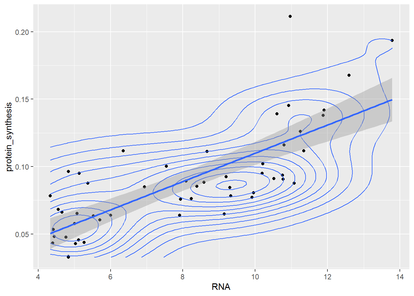
Notice that the different layers of the plot gets added on top of each other in the order that we mention them in the code.
Two-dimensional visualizations can of course combine a categorical variable with a continous variable. In the next plot we use another familiar geometric representation, the boxplot.
ggplot(data = millward, aes(group, protein_synthesis)) +
  geom_boxplot()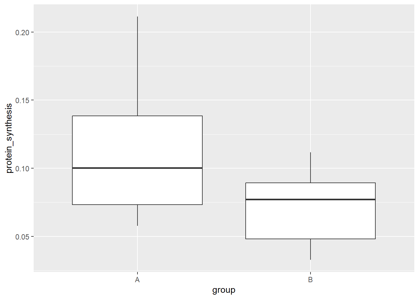
The continous variable can be displayed as individual data points. Using geom_point with a categorical variable on the x-axis gives us a transparent display of the data.
ggplot(data = millward, aes(group, protein_synthesis)) +
  geom_point()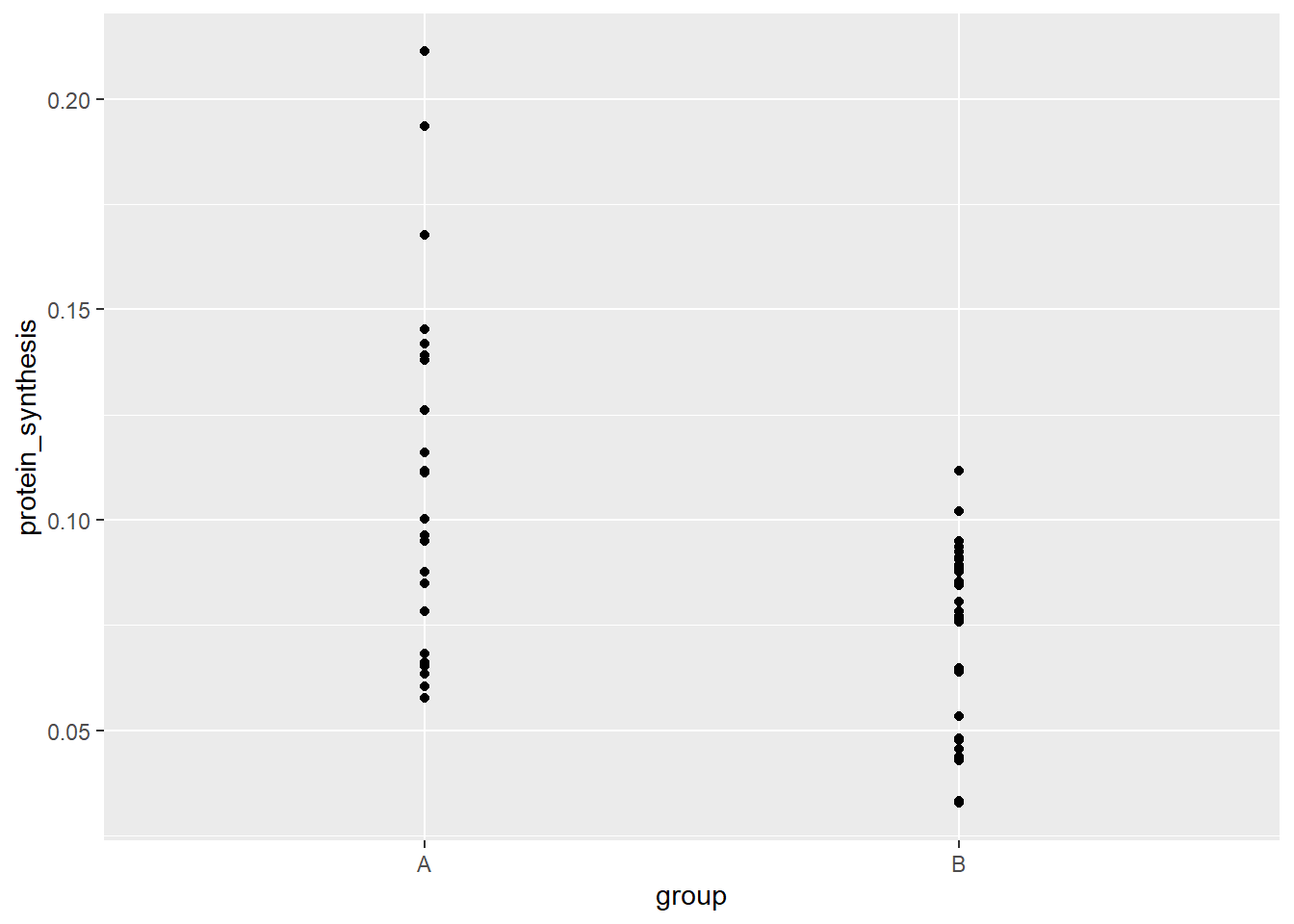
When we have many data points we might have overplotting. In a grouped figure, like the one above we can use another geom that adresses this.
ggplot(data = millward, aes(group, protein_synthesis)) +
  geom_jitter(width = 0.1)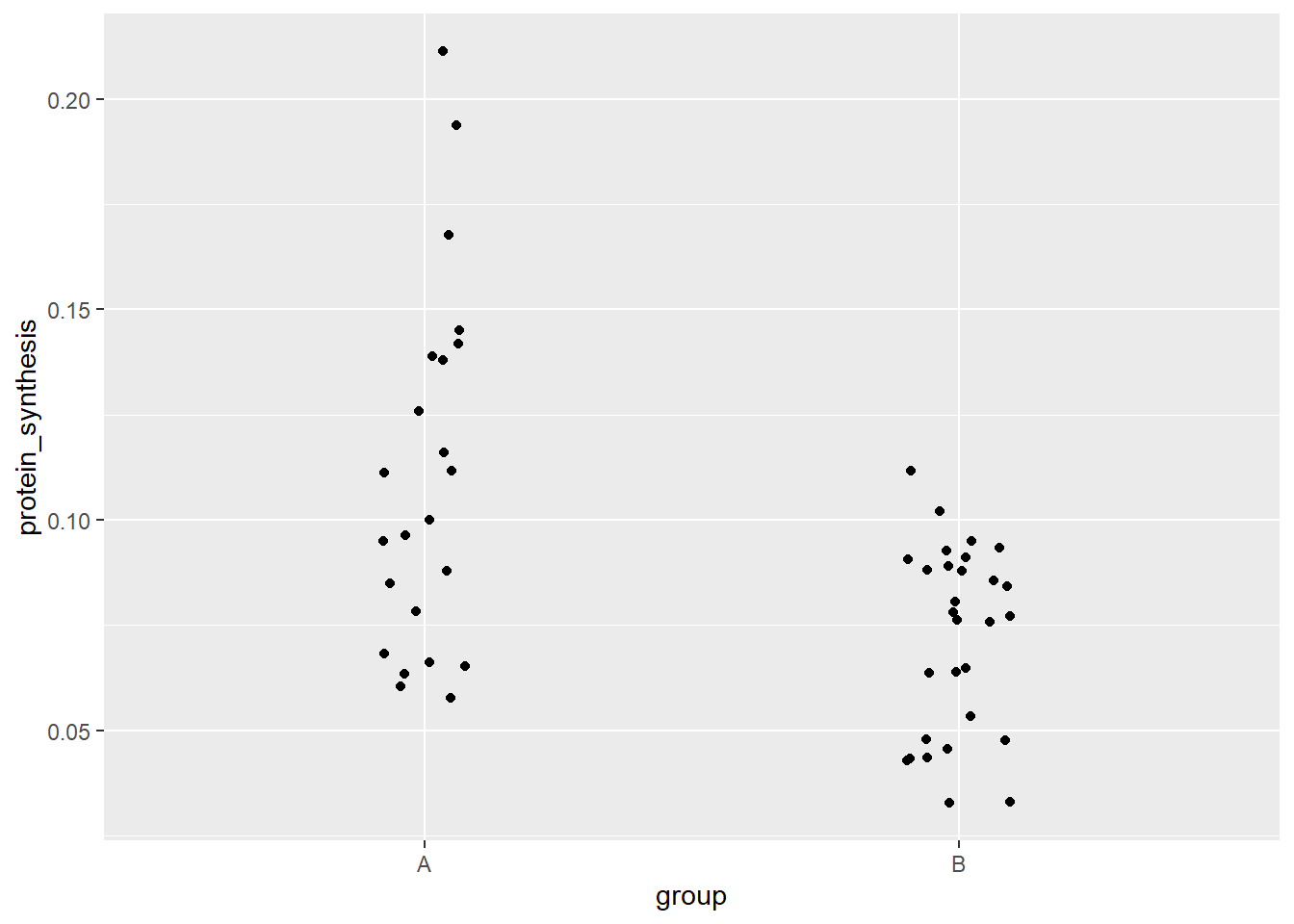
Notice that I’ve used width = 0.1 to reduce the spread of the data points. geom_jitter adds some noise in the horizontal plane but retains the point position in the vertical plane. The added noise makes it possible to avoid overplotting. Another alternative is a dotplot, adding gentle binning of the data points on the y-axis avoids overplotting and gives a good sense of the spread in each group. Again, notice in the code below, we are using some geom-specific settings to customize the default.
ggplot(data = millward, aes(group, protein_synthesis)) +
  geom_dotplot(binaxis = "y", stackdir = "center")
Bin width defaults to 1/30 of the range of the data. Pick better value with
`binwidth`.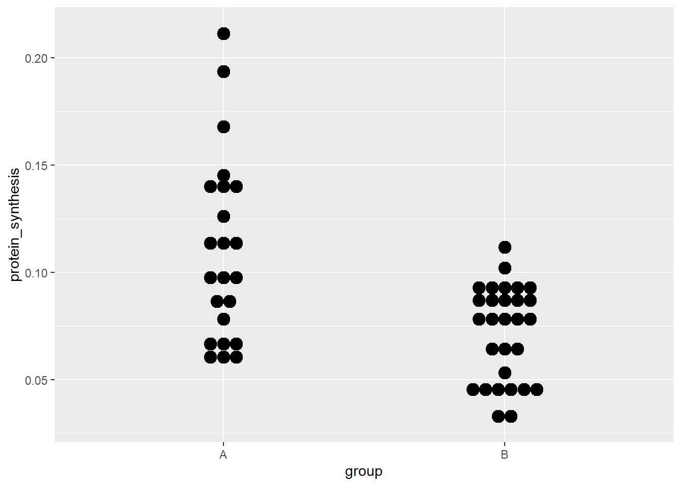
There are many more alternatives for two-dimensional displays, we will explore customizations below.
5.3.3 Multi-dimensional visualizations
We so far used the coordinate system to display two variables, either as the raw data (geom_point) or after some data transformation to represent e.g., counts. We can add dimension, or variables to our graph by using some of the other available aesthetics.
Let’s combine the grouping variable to the scatterplot as determining the color. By defining a variable for the color argument we tell ggplot2 to add colors by group to all subsequent geoms.
ggplot(data = millward, aes(RNA, protein_synthesis, color = group)) +
  geom_point()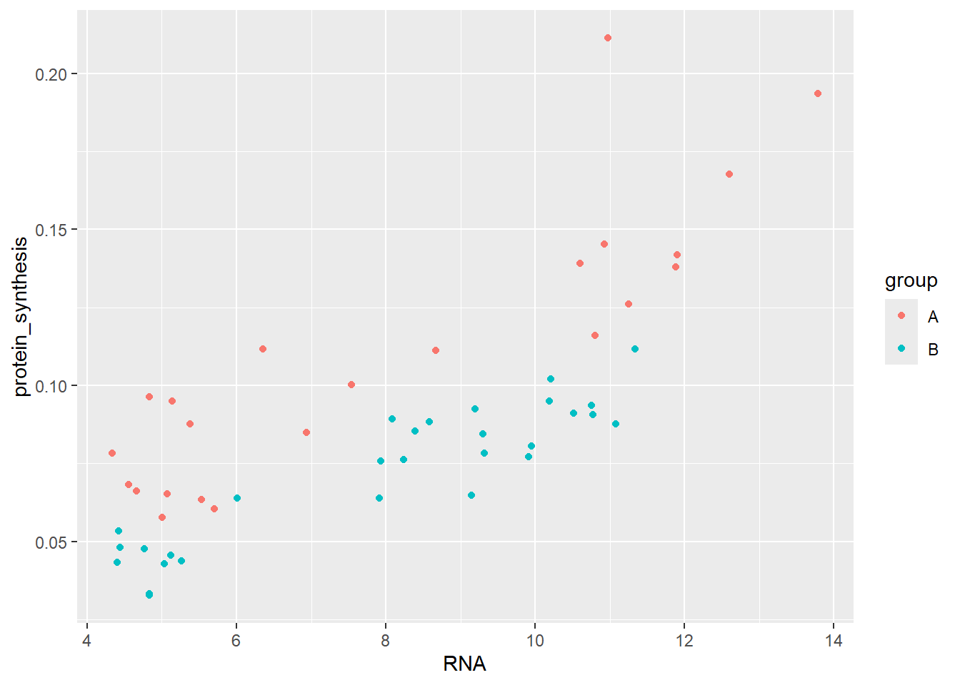
We have effectively introduced “another dimension” into the figure. We could also use shape to separate the groups while still usig the default points geom.
ggplot(data = millward, aes(RNA, protein_synthesis, shape = group)) +
  geom_point()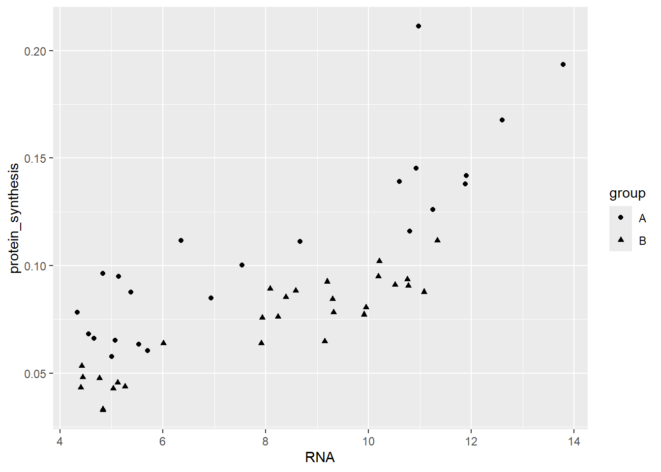
Furthermore, the group variable could be mapped to several aestetics.
ggplot(data = millward, aes(RNA, protein_synthesis,
                            shape = group,
                            color = group)) +
  geom_point()
Different geoms have different capabilities to convey aesthetics, see for example ?geom_point under Aesthetics.
An alternative to points are labels and text. geom_label creates labels at the specified x- and y-coordinates.
ggplot(data = millward, aes(RNA, protein_synthesis, label = group)) +
  geom_label()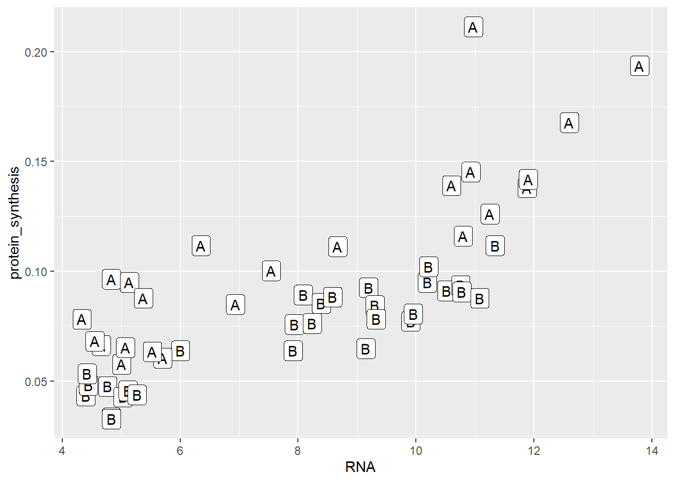
Similarly to geom_label, geom_text adds the data in the group variable to specified coordinates, however without the label background. Go ahed and explore the difference for your self.
5.3.4 Dividing graphs into subplots using data variables
Another alternative to using geoms to distinguish discrete (categorical) levels is to use facets. Facets will use a variable in the data for creating two or more panels. facet_wrap(~ group) will for example give us two panels, one for each group.
ggplot(data = millward, aes(RNA, protein_synthesis)) +
  geom_point() +
  facet_wrap( ~ group)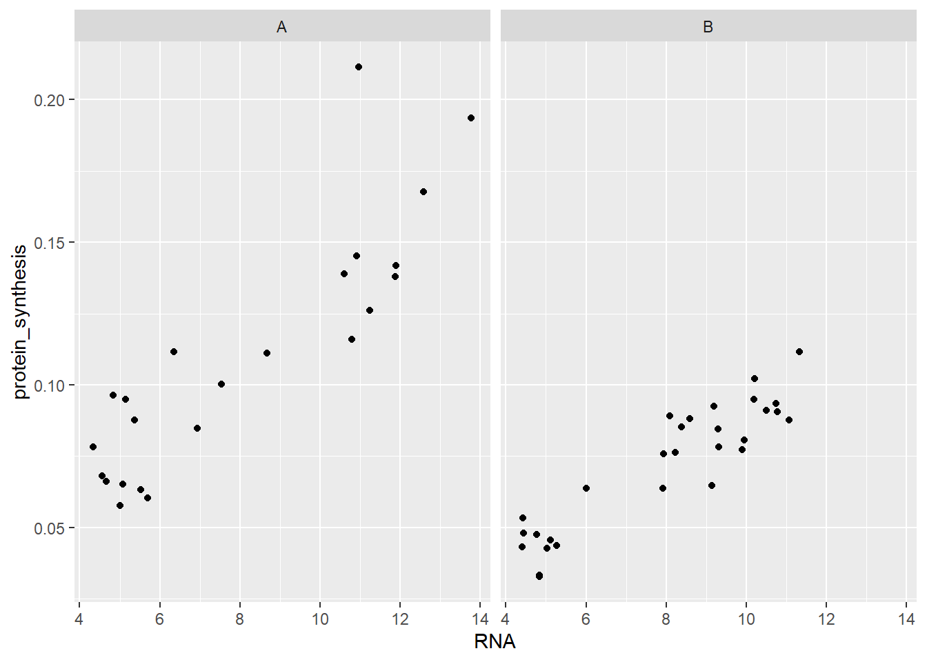
Notice that the scales (x- and y-axis) remains the same in both panels. We could change this behaviour by adding scales = "free"
ggplot(data = millward, aes(RNA, protein_synthesis)) +
  geom_point() +
  facet_wrap( ~ group, scales = "free")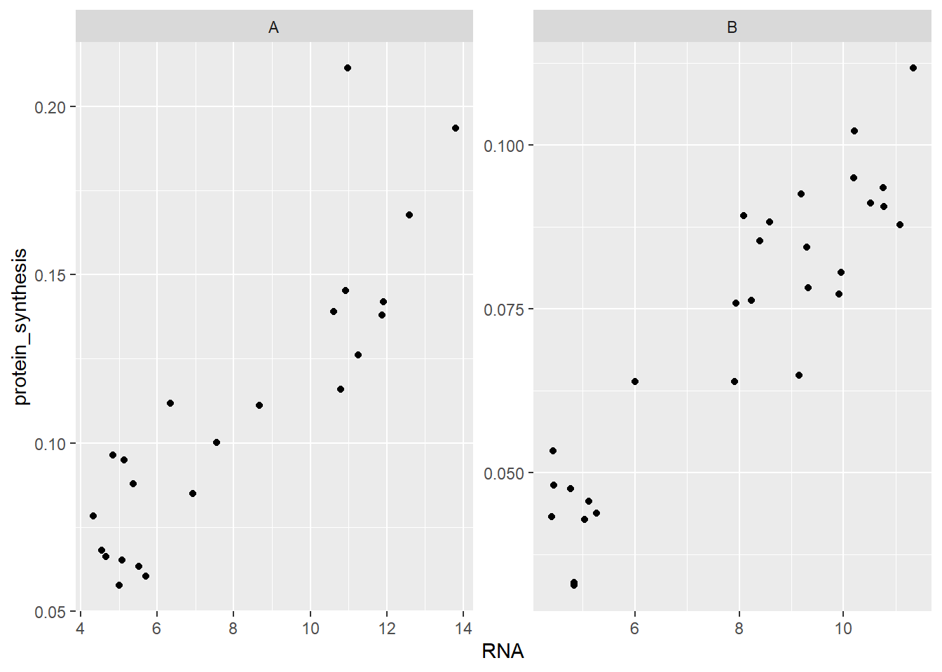
facet_grid is another alternative for creating panels. The syntax for facet_grid expects to categorical variables, if only one is needed we can use a . on one side of the ~ (tilde) symbol. The ~ separates rows and columns, setting facet_grid(group ~ .) gives us two panels where the group variable seperates in rows.
ggplot(data = millward, aes(RNA, protein_synthesis)) +
  geom_point() +
  facet_grid( group ~ . )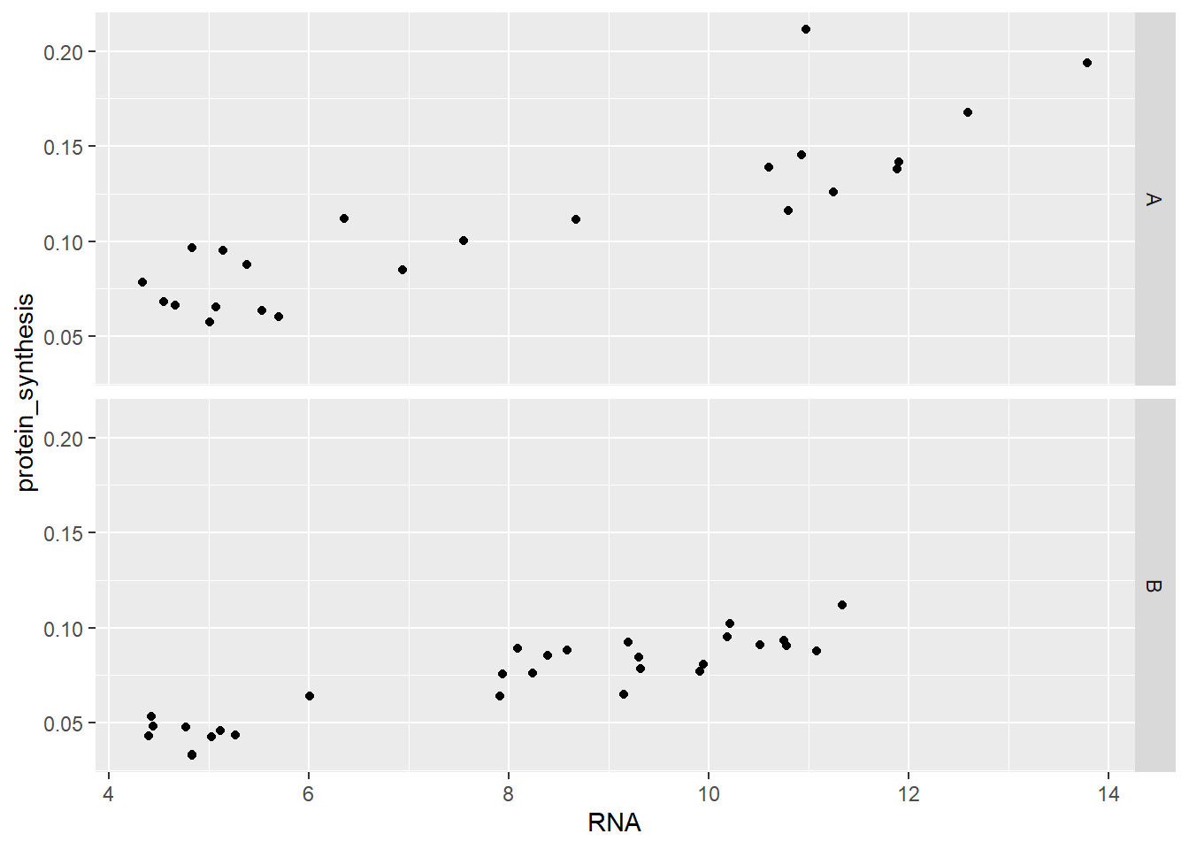
5.4 Beyond defaults: Scales, labels, annotations and themes
So far we have used data to generate basic visualizations. ggplot2 creates these visualizations using many default design decisions and names of variables available in the data. This is not always what we need. In this section we will explore how to customize our data visualization.
5.4.1 Scales
We can modify the way data is mapped to coordinates or geometric objects in a ggplot. This is done by changing the scales of an aesthetic. As an example, we might want to control what shapes are being mapped to each level of a category variable. Using scale_shape_manual(values = c(21, 22)) we specify that the values (shapes) should be number 21 and 22. These shapes will be applied to the levels of the categorical variable in the specified order (Figure 5.27).
Code
library(patchwork)

a <- ggplot(data = millward, aes(RNA, protein_synthesis, shape = group)) +
  geom_point() +
  labs(subtitle = "Default scale")

b <- ggplot(data = millward, aes(RNA, protein_synthesis, shape = group)) +
  geom_point() +
  scale_shape_manual(values = c(21, 22))  +
  labs(subtitle = "scale_shape_manual(values = c(21,22))")


a | b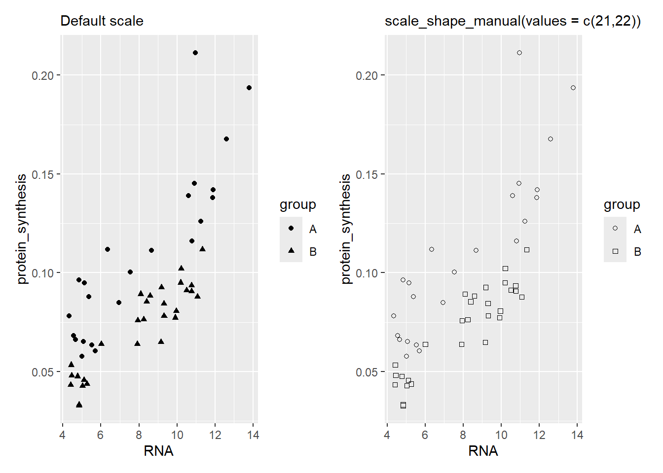
We could also change the scale of the ccordinate system. Using scale_x_continous and scale_y_continous we get access to several options for the x- and y-coordinate scales. Let’s say we want to include 0 and control the breaks in the scale.
ggplot(data = millward, aes(RNA, protein_synthesis)) +
  geom_point() +
  scale_x_continuous(limits = c(0, 15),
                     breaks = c(0, 5, 10, 15),
                     expand = c(0, 0)) +

  scale_y_continuous(limits = c(0, 0.25),
                     breaks = c(0, 0.05, 0.10, 0.15, 0.2, 0.25),
                     expand = c(0, 0))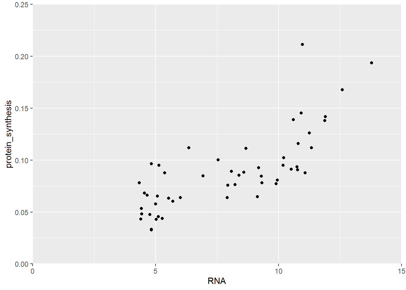
In Figure 5.28 we extended the scales all the way dow to 0 and fixed the upper limits and breaks.
Fills and colors are also possible to control using special scale functions. Let’s say we are using colors to separate the two groups. We might want to control what colors are being mapped to each group. We can do this by using the “manual” scaling function. Here we provide hexadecimal color codes representing two colors.
ggplot(data = millward, aes(RNA, protein_synthesis, color = group)) +
  geom_point(size = 3)  +
  scale_color_manual(values = c("#FF2344", "#123456"))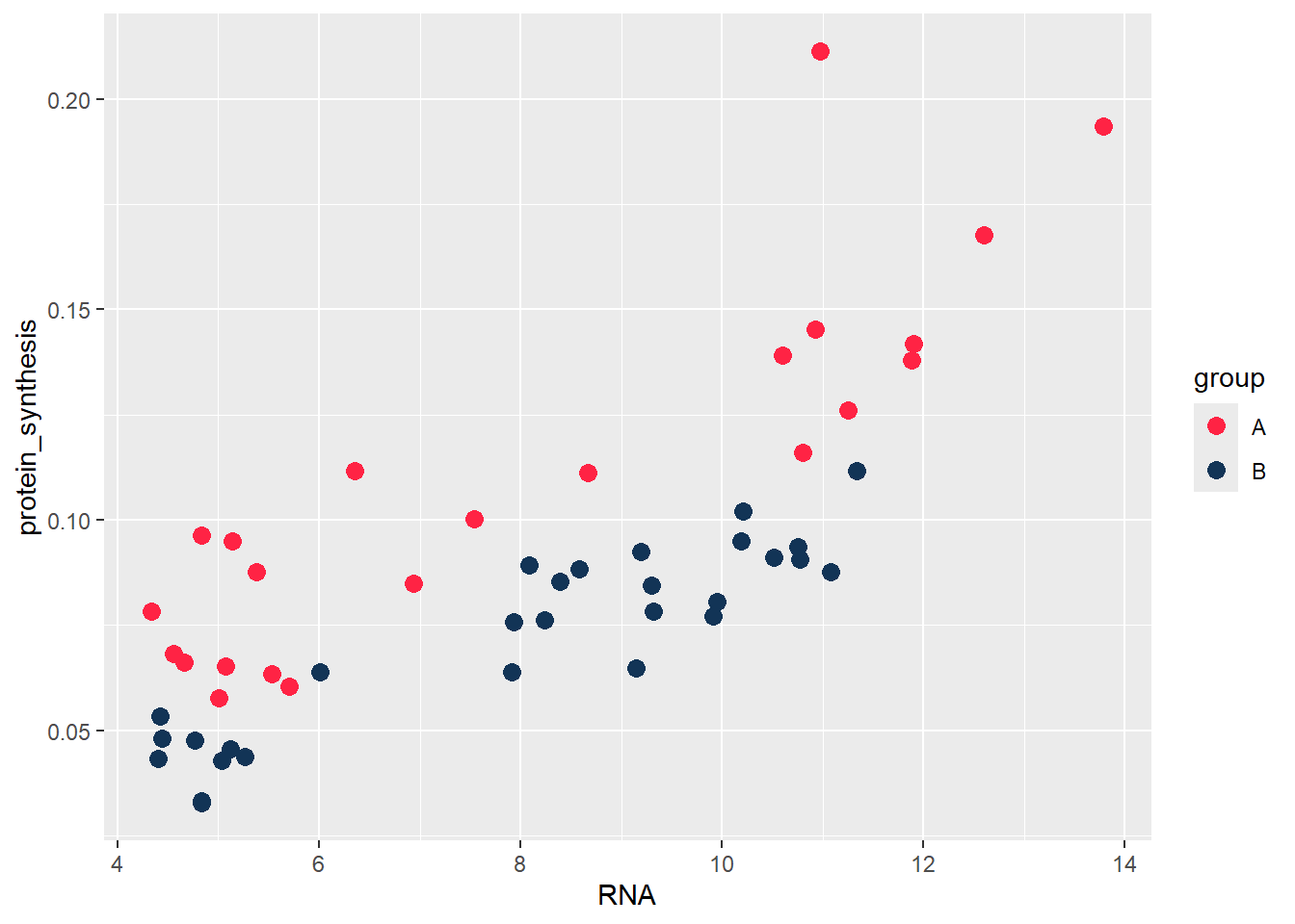
ggplot2 has several built in color/fill scales that can be useful. For example, when changing our color scale function to scale_color_brewer we can use a discrete color set where colors have been selected based on compability (see colorbrewer2).
ggplot(data = millward, aes(RNA, protein_synthesis, color = group)) +
  geom_point(size = 3)  +
  scale_color_brewer(palette = "Dark2")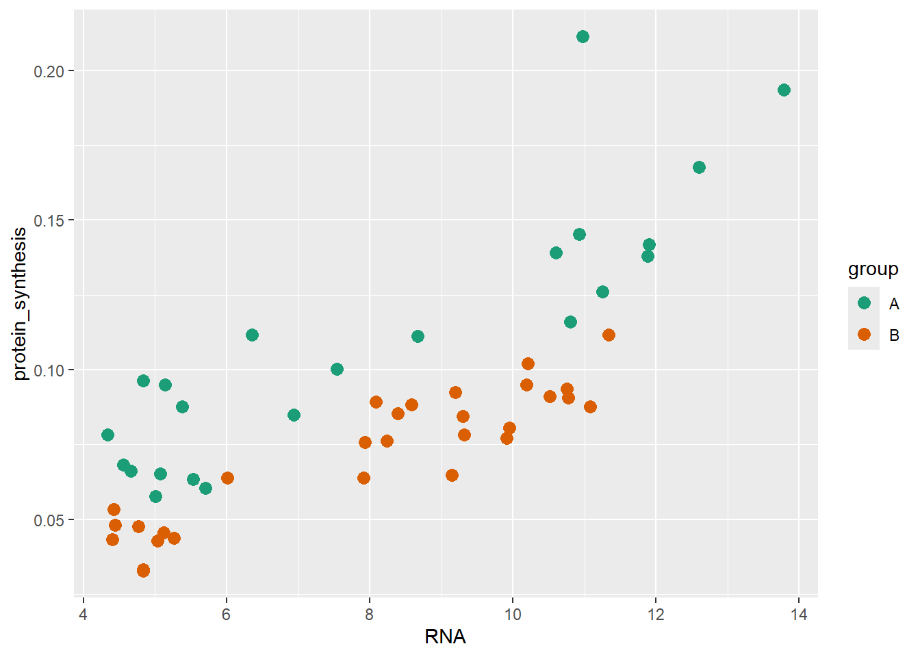
Color and fill can also be mapped to continuous values, and we can controll this behavior by using scale functions. In the plot below we are going back to a previous example where we mapo group to the x-axis and protein synthesis to the y-axis. Additionally, we use a continouos fill scale to map the RNA variable.
ggplot(data = millward, aes(group, protein_synthesis, fill = RNA)) +
  geom_jitter(size = 3, shape = 21, width = 0.1)  +
  scale_fill_continuous()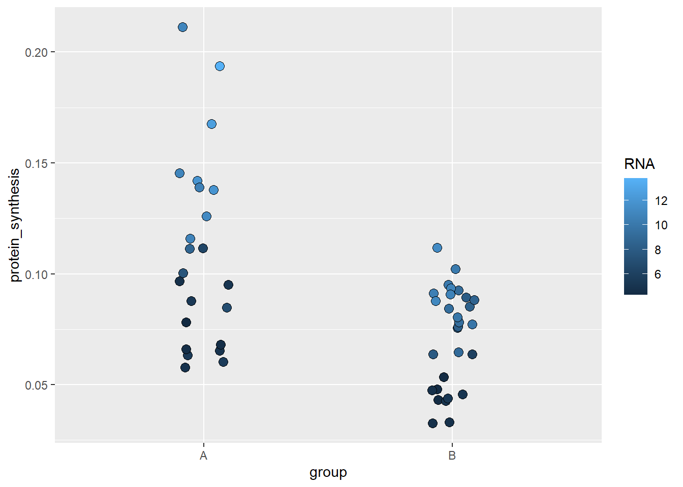
The default in scale_fill_continuous can be manipulated using your own gradient which will create a scale between two end-points of your selection.
ggplot(data = millward, aes(group, protein_synthesis, fill = RNA)) +
  geom_jitter(size = 3, shape = 21, width = 0.1)  +
  scale_fill_gradient(low = "red", high = "yellow")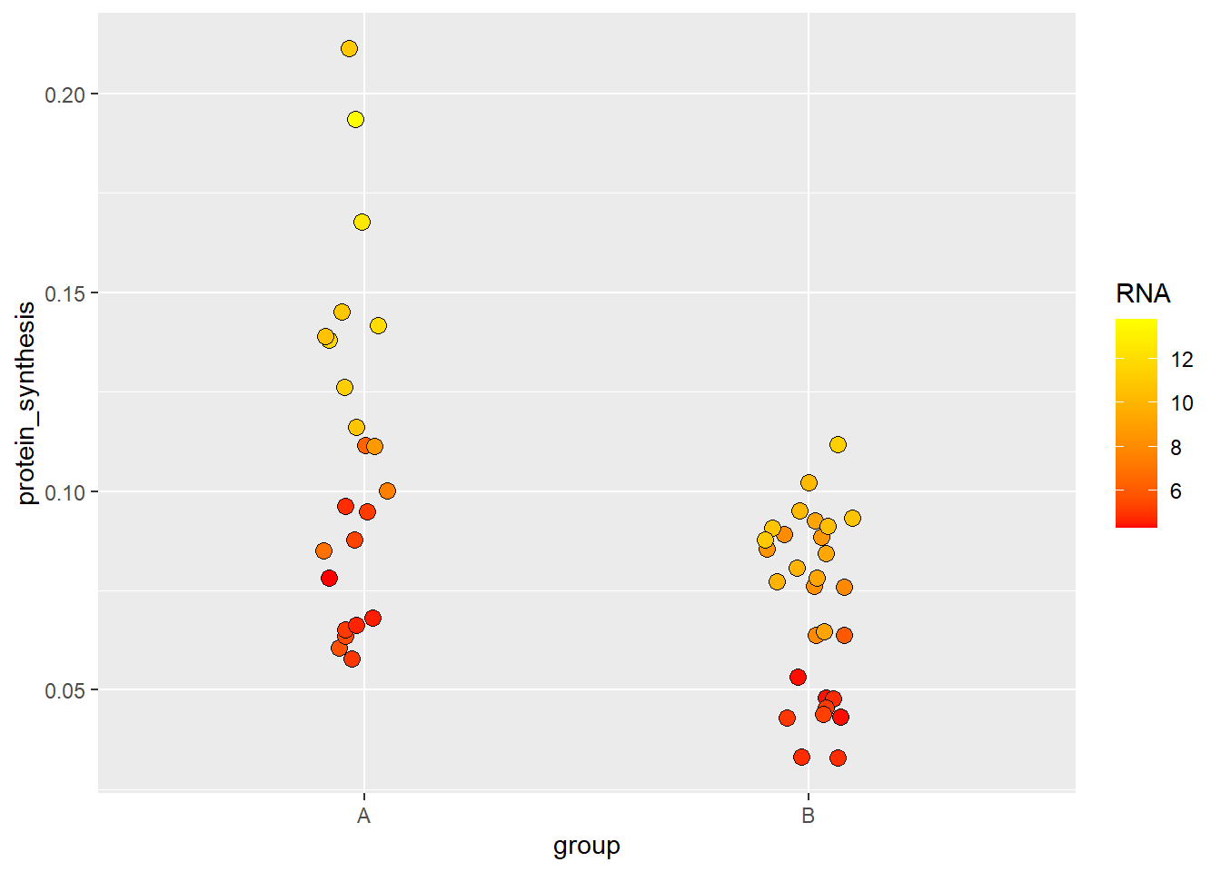
As we have seen above, there are several specialized function for controlling scales onto data is being mapped. All aesthetics have specialized function making ggplot2 very flexible. See the ggplot2 reference on scales for more details.
5.4.2 Labels
Labels are automatically created in ggplot2 using variable names. Most often we need to provide more information to the consumer of our figure in order for it to make sense. We can change what is being displayed by simply overriding the default behaviour of naming e.g., axes by variable names.
ggplot(data = millward, aes(group, protein_synthesis, fill = RNA)) +
  geom_jitter(size = 3, shape = 21, width = 0.1)  +
  scale_fill_gradient(low = "red", high = "yellow") +

  labs(x = "Experimental group",
       y = "Protein synthesis (ks, day-1)",
       fill = "RNA content (ug mg-1)")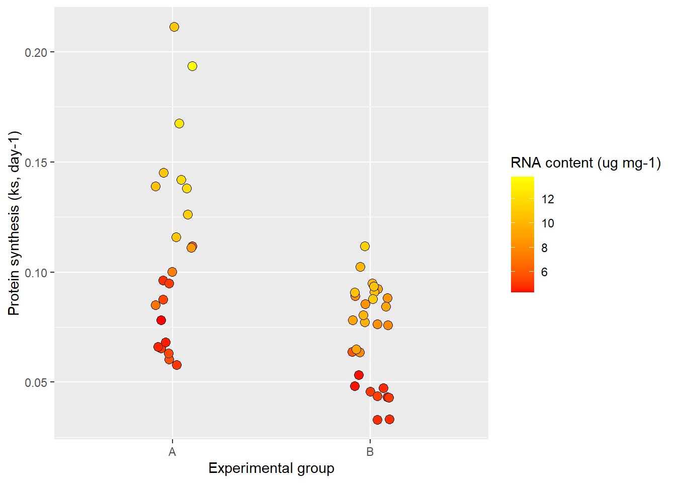
The labsfunction let’s us decide labels for each aesthetic. Notice that I included a label for the fill also which controls the title for the legend.
To get even more control of our labels we want to be able to include special characters subscript and superscript. Ideally the y-axis should be “Protein synthesis (ks, day-1)” and the fill label should be “RNA content (μg mg-1)”. This is possible using plotmath syntax.
ggplot(data = millward, aes(group, protein_synthesis, fill = RNA)) +
  geom_jitter(size = 3, shape = 21, width = 0.1)  +
  scale_fill_gradient(low = "red", high = "yellow") +

  labs(x = "Experimental group",
       y = expression("Protein synthesis (" * k[s] * ", day" ^-1 * ")"),
       fill = expression("RNA content (" * mu * "g mg" ^-1 * ")"))
I find the plotmath system a bit confusing and often resort to using the ggtext package which is a package that allows markdown syntax. For this to work we need to have the ggtext package installed and change tell ggplot2 that the label text is a special case. In the example below I’m using markdown syntax to customize the label text and the theme function to specify the type of element needed for correct interpretation of the markdown syntax. The element_markdown functions comes from ggtext and helps ggplot2 to translate the markdown syntax.
library(ggtext)
ggplot(data = millward, aes(group, protein_synthesis, fill = RNA)) +
geom_jitter(size = 3, shape = 21, width = 0.1) +
scale_fill_gradient(low = "red", high = "yellow") +
labs(x = "Experimental group",
y = "Protein synthesis, (k<sub>s</sub>, day<sup>−1</sup>)",
fill = "RNA content (μg mg<sup>-1</sup>)") +
theme(axis.title.y = element_markdown(),
legend.title = element_markdown())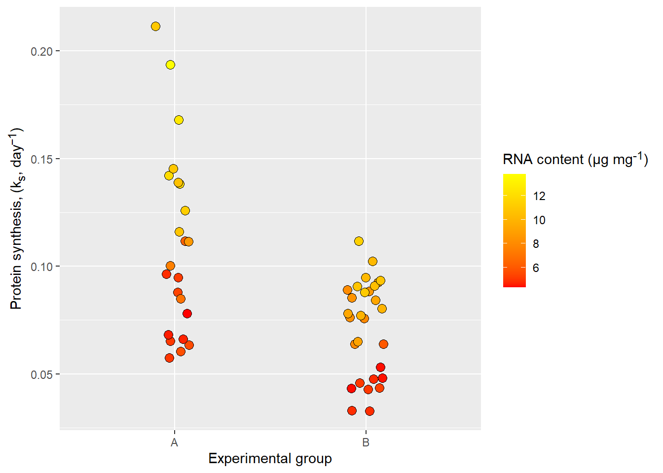
ggtext.
Notice that some text aspects might need some tweeking, using the html code for the minus sign seems to work bettwer for vertically oriented axis titles. Flexibility often comes with additional complexity.
5.4.3 Annotations
Annotations are non-data layers of a graph that can diect attention to special details of the plot. For example we might want to highlight an observation or add statistics from a comparison between groups. This can be accomplished with annotations.
library(ggtext)
# Calculate statistics and extract the p-value
mod <- lm(protein_synthesis ~ group, data = millward)
pval <- round(coef(summary(mod))[2,4], 5)
ggplot(data = millward, aes(group, protein_synthesis, fill = RNA)) +
geom_jitter(size = 3, shape = 21, width = 0.1) +
scale_fill_gradient(low = "red", high = "yellow") +
scale_y_continuous(limits = c(0, 0.3),
expand = c(0, 0),
breaks = c(0, .10, .20, .30)) +
labs(x = "Experimental group",
y = "Protein synthesis, (k<sub>s</sub>, day<sup>−1</sup>)",
fill = "RNA content (μg mg<sup>-1</sup>)") +
theme(axis.title.y = element_markdown(),
legend.title = element_markdown()) +
# Annotation layers for comparison
annotate("segment", x = 1, xend = 2, y = 0.25, yend = 0.25) +
annotate("segment",
x = c(1, 2),
xend = c(1, 2),
y = c(0.25, 0.25),
yend = c(0.24, 0.24) ) +
annotate("text", label = paste0("P-value = ", pval),
x = 1.5, y = 0.26) +
# Annotation layer for highlighting
annotate("curve", x = 2.2, xend = 2, y = 0.18, yend = 0.12, curvature = 0.3,
arrow = arrow(type = "closed", length = unit(2.5, "mm"))) +
annotate("text", x = 2.2, y = 0.19, label = "Highlight")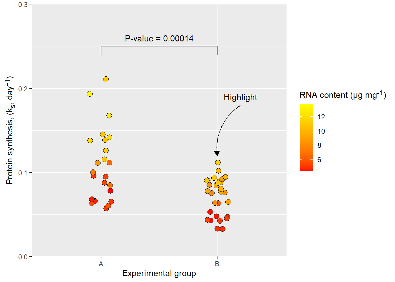
The annotate function can use any geom with its available option to create annotation layers.
5.4.4 Themes
We have already used the theme function to declare a specific element type (element_markdown for label text). The theme function contains options that can change the apperance of visual elemnts of the graph not determined by data, scales or annotations.
There are a number of pre-specified themes in ggplot2, these themes contain matching customizations of visual elements making them a good starting point for further customizations (see Figure 5.37).
Code
p <- ggplot(data = millward, aes(group, protein_synthesis, fill = RNA)) +
geom_jitter(size = 3, shape = 21, width = 0.1) +
scale_fill_gradient(low = "red", high = "yellow") +
scale_y_continuous(limits = c(0, 0.3),
expand = c(0, 0),
breaks = c(0, .10, .20, .30)) +
labs(x = "Experimental group",
y = "Protein synthesis, (k<sub>s</sub>, day<sup>−1</sup>)",
fill = "RNA content (μg mg<sup>-1</sup>)") +
theme(axis.title.y = element_markdown(),
legend.title = element_markdown()) +
# Annotation layers for comparison
annotate("segment", x = 1, xend = 2, y = 0.25, yend = 0.25) +
annotate("segment",
x = c(1, 2),
xend = c(1, 2),
y = c(0.25, 0.25),
yend = c(0.24, 0.24) ) +
annotate("text", label = paste0("P-value = ", pval),
x = 1.5, y = 0.26) +
# Annotation layer for highlighting
annotate("curve", x = 2.2, xend = 2, y = 0.18, yend = 0.12, curvature = 0.3,
arrow = arrow(type = "closed", length = unit(2.5, "mm"))) +
annotate("text", x = 2.2, y = 0.19, label = "Highlight")
(p +
labs(title = "Default theme") +
theme(axis.title.y = element_markdown(),
legend.title = element_markdown()) |
p + theme_bw() +
labs(title = "theme_bw()") +
theme(axis.title.y = element_markdown(),
legend.title = element_markdown()) ) /
(p + theme_linedraw() +
labs(title = "theme_linedraw()") +
theme(axis.title.y = element_markdown(),
legend.title = element_markdown()) |
p + theme_light() +
labs(title = "theme_light()") +
theme(axis.title.y = element_markdown(),
legend.title = element_markdown()) ) /
(p + theme_dark() +
labs(title = "theme_dark()") +
theme(axis.title.y = element_markdown(),
legend.title = element_markdown()) |
p + theme_minimal() +
labs(title = "theme_minimal()") +
theme(axis.title.y = element_markdown(),
legend.title = element_markdown()) ) /
(p + theme_classic() +
labs(title = "theme_classic()") +
theme(axis.title.y = element_markdown(),
legend.title = element_markdown()) |
p + theme_void() +
labs(title = "theme_void()") +
theme(axis.title.y = element_markdown(),
legend.title = element_markdown()) )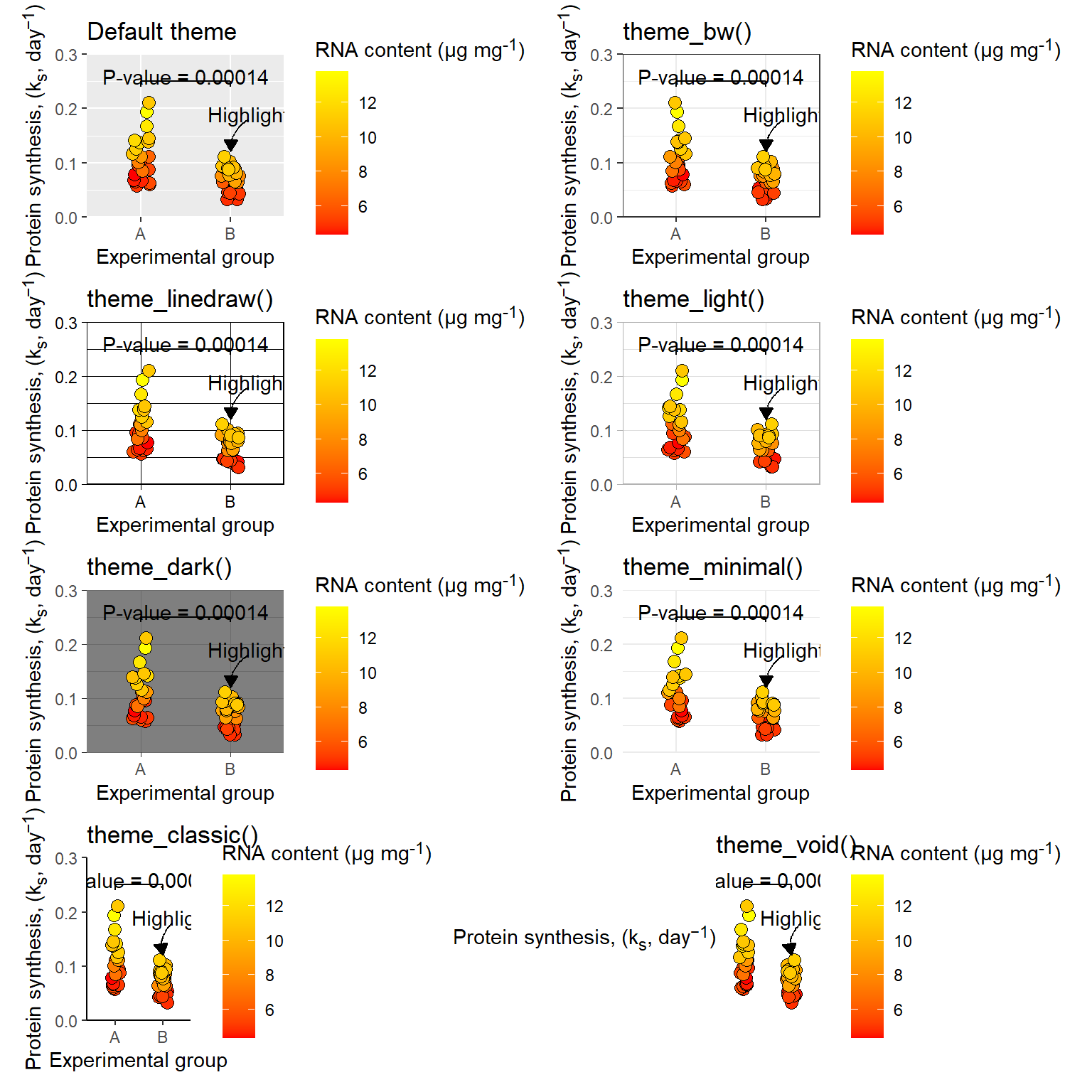
Changing aspects of a theme is done using element functions that are used to control figure elements. For example plot.title is an element of a ggplot2 figure, it is controled by the element_text function.
p <- ggplot(data = millward, aes(group, protein_synthesis, fill = RNA)) +
geom_jitter(size = 3, shape = 21, width = 0.1) +
scale_fill_gradient(low = "red", high = "yellow") +
scale_y_continuous(limits = c(0, 0.3),
expand = c(0, 0),
breaks = c(0, .10, .20, .30)) +
labs(x = "Experimental group",
y = "Protein synthesis, (k<sub>s</sub>, day<sup>−1</sup>)",
fill = "RNA content (μg mg<sup>-1</sup>)",
title = "This title has been customized") +
# Annotation layers for comparison
annotate("segment", x = 1, xend = 2, y = 0.25, yend = 0.25) +
annotate("segment",
x = c(1, 2),
xend = c(1, 2),
y = c(0.25, 0.25),
yend = c(0.24, 0.24) ) +
annotate("text", label = paste0("P-value = ", pval),
x = 1.5, y = 0.26) +
# Annotation layer for highlighting
annotate("curve", x = 2.2, xend = 2, y = 0.18, yend = 0.12, curvature = 0.3,
arrow = arrow(type = "closed", length = unit(2.5, "mm"))) +
annotate("text", x = 2.2, y = 0.19, label = "Highlight") +
# Theme customization
theme(plot.title = element_text(color = "red"),
axis.title.y = element_markdown(),
legend.title = element_markdown())
p 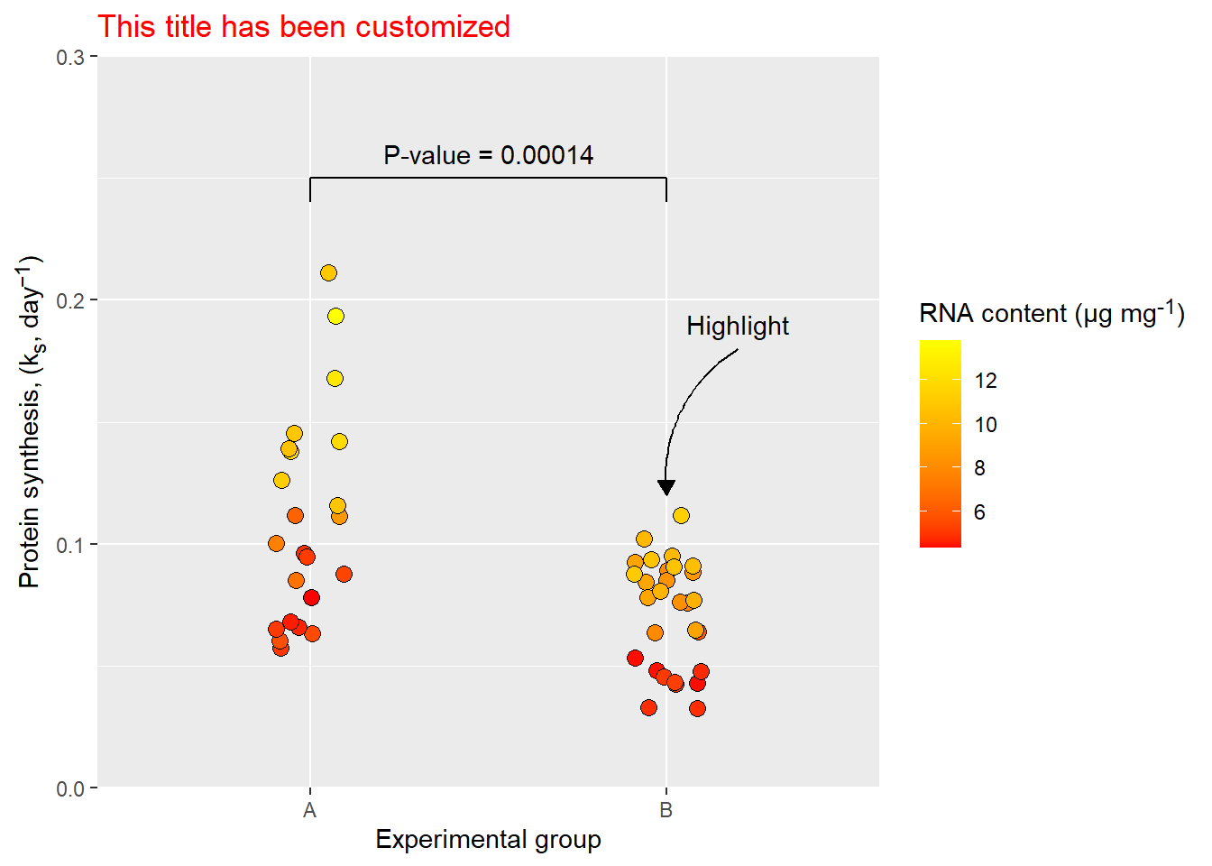
In addition to text elements (adjustable with element_text and element_markdown) we have can customize line elements with element_line and rectangular elements with element_rect. For example, the plot background is a rectangular element which can be medified with fill, color, linewidth and linetype.
p + theme(plot.background = element_rect(fill = "lightblue",
                                         color = "darkblue",
                                         linewidth = 2,
                                         linetype = "dashed"))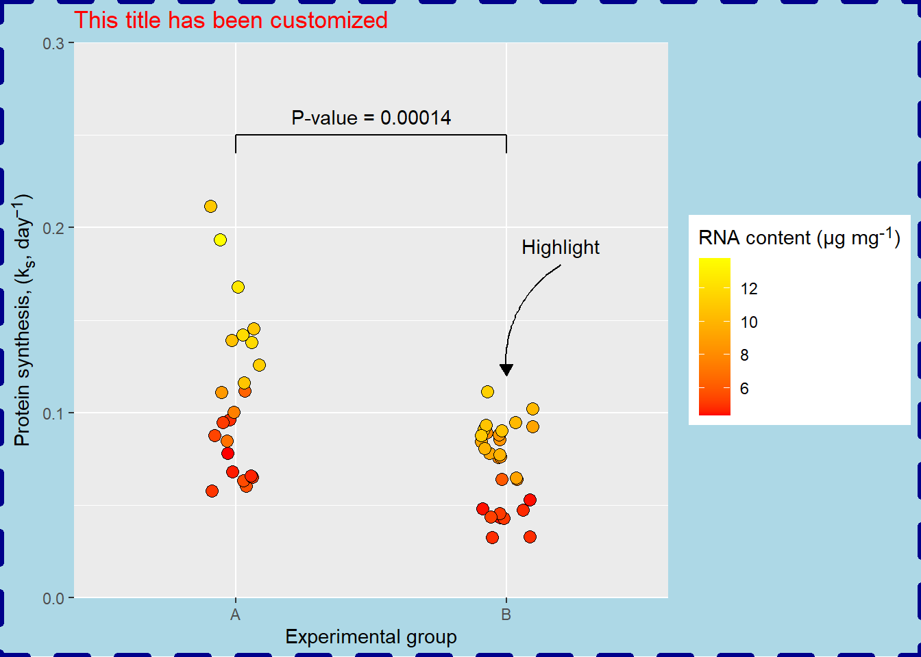
The grid lines (panel.grid.major) are elements controlled by element_line. element_line takes arguments to control color, linewidth, linetype, lineend and arrow. To create an example we will try to make silly customizations to all of these options.
p + theme(panel.grid.major = element_line(
                                         color = "darkblue",
                                         linewidth = 2,
                                         arrow = arrow(type = "closed"),

                                         linetype = "dashed",
                                         lineend = "round"))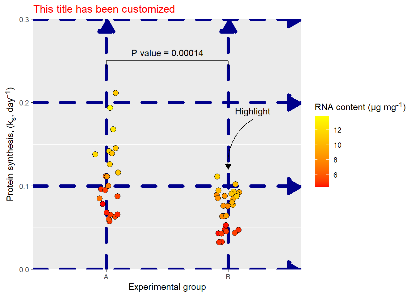
Finally, element_blank removes a theme element. This is useful when we do not want to display a certain element of a graph.
The theme function is also where we specify positioning of the legend. The legend will contain a representation of the scale of any data mapped to aesthetics other than x- and y-coordinates. We might want to remove it (legend.position = "none") or place it at at the "left", the “right”, the "bottom", or at the "top" of the plot area. When specifying "inside" we also need to set the position inside the plotting area (legend.position.inside). In the example below, I’m also setting the legend direction to horizontal in the “inside” version. This option is implicitly set using legend.position = "bottom".
Code
# The basic plot, saved in p
p <- ggplot(data = millward, aes(group, protein_synthesis, fill = RNA)) +
geom_jitter(size = 3, shape = 21, width = 0.1) +
scale_fill_gradient(low = "red", high = "yellow") +
scale_y_continuous(limits = c(0, 0.4),
expand = c(0, 0),
breaks = c(0, .10, .20, .30)) +
labs(x = "Experimental group",
y = "Protein synthesis, (k<sub>s</sub>, day<sup>−1</sup>)",
fill = "RNA content (μg mg<sup>-1</sup>)") +
# Annotation layers for comparison
annotate("segment", x = 1, xend = 2, y = 0.25, yend = 0.25) +
annotate("segment",
x = c(1, 2),
xend = c(1, 2),
y = c(0.25, 0.25),
yend = c(0.24, 0.24) ) +
annotate("text", label = paste0("P-value = ", pval),
x = 1.5, y = 0.27) +
# Annotation layer for highlighting
annotate("curve", x = 2.2, xend = 2, y = 0.18, yend = 0.12, curvature = 0.3,
arrow = arrow(type = "closed", length = unit(2.5, "mm"))) +
annotate("text", x = 2.2, y = 0.19, label = "Highlight") +
# Theme customization
theme(axis.title.y = element_markdown(),
legend.title = element_markdown())
a <- p +
theme(legend.position = "inside",
legend.position.inside = c(0.5, 0.9),
legend.direction = "horizontal") +
labs(subtitle = "legend.position = 'inside'")
b <- p +
theme(legend.position = "bottom",
legend.position.inside = c(0.8, 0.8)) +
labs(subtitle = "legend.position = 'bottom'")
a|b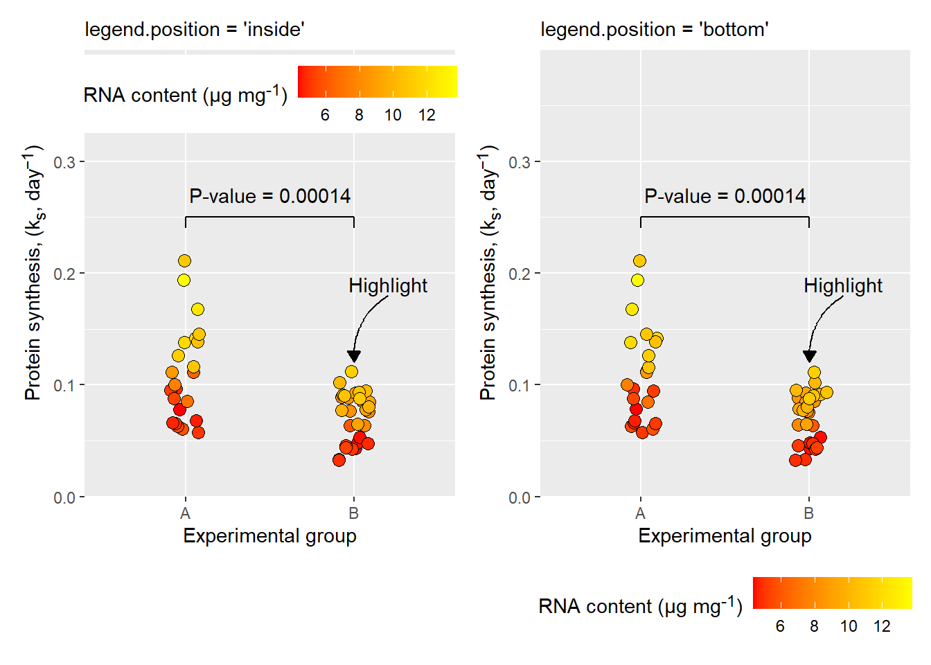
The legend placement customization is an example of theme options that do not use special element functions.
There are more than 130 options available for customization in the theme function, many of which inherits from others in a hierarchy. For example, axis.title.x inherits options from the above level axis.title, which inherits from the upper level text. Specifying options in text will affect lower level options if they are not explicitly set.
For a complete overview of theme components, see the ggplot2 reference.
5.4.5 Using or creating a custom theme
You might not want to get stuck using the themes available in ggplot2. Do not worry, the R/ggplot2 community has been really productive creating custom themes. The ggthemes package contains several custom themes, so does tvthemes, another package containing custom themes.
If you want to create you own theme that can be reused across different plots, all you need to do is to specify a function containing the theme settings. In the example below I’m take advantage of theme_classic() and add customizations for my own theme. Adding this theme to my plot will update it with my theme settings. This makes custom themes easily reusable.
theme_myown <- function() {

  theme_classic() +
    theme(plot.background = element_rect(fill = "lightblue"),
          text = element_text(color = "darkblue"),
          axis.title.y = element_markdown(),
          legend.title = element_markdown())


}


p / p + theme_myown() 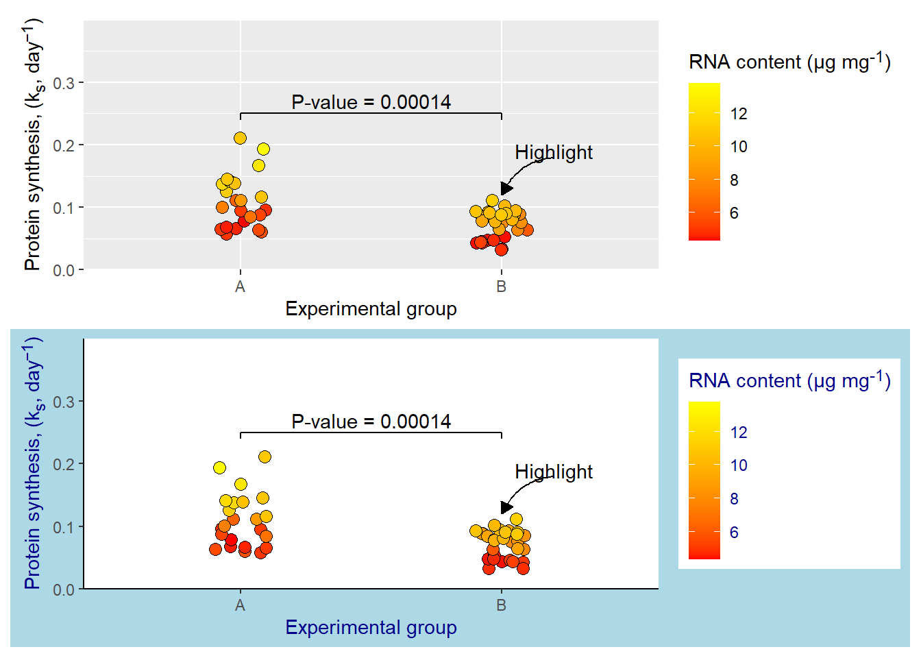
5.5 Combining plots
We might want to create figures that contain several panels. As we have seen, creating multipanel plots is easy using the facet_* functionality. But this is not possible when we use different data, or different types of x- and y-coordinate specifications.
There are several options for combining two different plots from ggplot2. One is patchwork, a package that provides a simple syntax for combining ggplot2 plots (and other graphics).
In the example below I’m creating two plots that I would like to arrange in a single multipanel plot, with panel annotations.
# Plot 1
p1 <- ggplot(data = millward, aes(group, protein_synthesis)) +
geom_jitter(size = 3, shape = 21, width = 0.1,
fill = "orange") +
scale_y_continuous(limits = c(0, 0.3),
expand = c(0, 0),
breaks = c(0, .10, .20, .30)) +
labs(x = "Experimental group",
y = "Protein synthesis, (k<sub>s</sub>, day<sup>−1</sup>)",
fill = "RNA content (μg mg<sup>-1</sup>)") +
theme_classic() +
# Annotation layers for comparison
annotate("segment", x = 1, xend = 2, y = 0.25, yend = 0.25) +
annotate("segment",
x = c(1, 2),
xend = c(1, 2),
y = c(0.25, 0.25),
yend = c(0.24, 0.24) ) +
annotate("text", label = paste0("P-value = ", pval),
x = 1.5, y = 0.26) +
# Theme customization
theme(axis.title.y = element_markdown(),
legend.title = element_markdown())
# Plot 2
p2 <- ggplot(data = millward, aes(RNA, protein_synthesis)) +
geom_point(size = 3, shape = 21, width = 0.1,
fill = "lightblue") +
theme_classic() +
labs(
y = "Protein synthesis, (k<sub>s</sub>, day<sup>−1</sup>)",
x = "RNA content (μg mg<sup>-1</sup>)") +
theme(axis.title.y = element_markdown(),
axis.title.x = element_markdown(),
legend.title = element_markdown()) Warning in geom_point(size = 3, shape = 21, width = 0.1, fill = "lightblue"):
Ignoring unknown parameters: `width`# Combining plots using patchwork syntax
(p1 | p2) + plot_annotation(tag_levels = "A")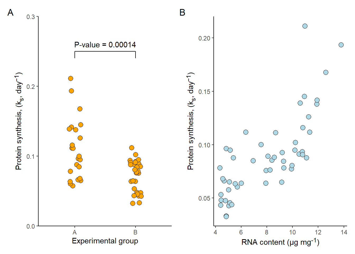
The syntax for patchwork is impressivly minimalistic. The bar (|) tells patchwork to combine the two plots on the same row. Combing the plots inside brachets makes it possible to add the plot_annotation(tag_levels = "A") which adds panel annotations to the combined figure.
Another package capable of combining figures into multipanel plots is cowplot. The workhorse function in cowplot is plot_grid.
library(cowplot)
Attaching package: 'cowplot'The following object is masked from 'package:patchwork':
align_plotsThe following object is masked from 'package:lubridate':
stampplot_grid(p1, p2,
align = "h",
labels = c("A", "B"))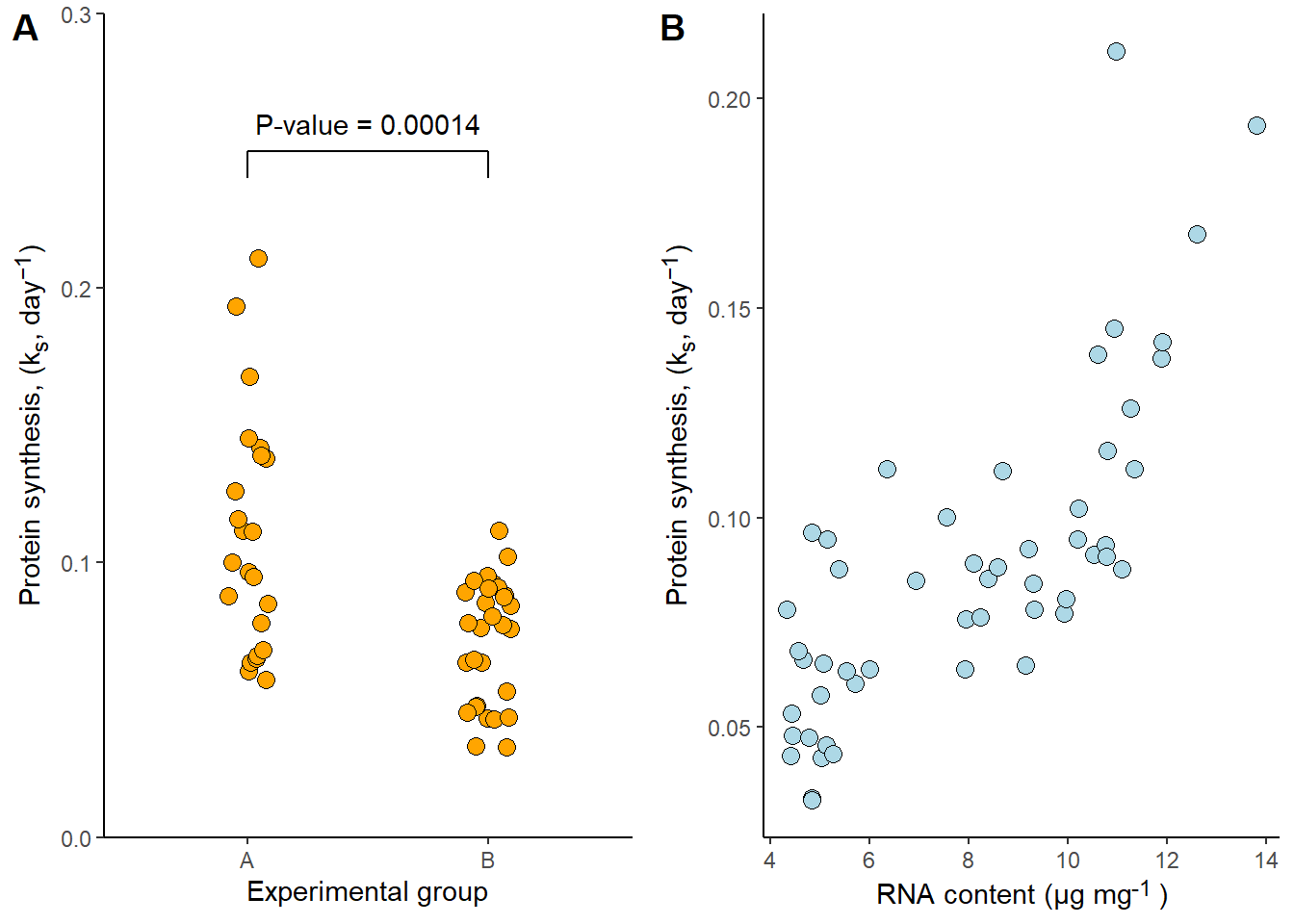
Both patchwork and cowplot are very well documented, flexible, and intuitive. They offer alot of additional features making it easy to combine several plots into a single figure.
5.6 Working with ggplot2 (and other plotting engines) in quarto
The quarto file format and software gives us the possibility to combine text with data-driven elements like figures and tables in several different output formats. To take full advantage of this functionality we need to use relevant chunk options.
A figure created using ggplot2 is defined inside a code chunk in a quarto file. A code chunk has several options relevant to including figures in a report. First, we need to tell quarto that the code chunk will produce a figure. Using the label option we define a label starting with the fig- prefix. Next, we might want to include a figure caption, this is done by defining the fig-cap option. If we are creating a report that includes a list of figures we might want to use a short caption, a short caption can be defined using fig-scap.
This small example would have a code chunk looking like this:
#| label: fig-examplequarto
#| fig-cap: "An example figure created as part of a report"
#| fig-scap: "A short example"
ggplot(data = millward, aes(RNA, protein_synthesis)) +
geom_point(size = 3, shape = 21,
fill = "lightblue") +
theme_classic() +
labs(
y = "Protein synthesis, (k<sub>s</sub>, day<sup>−1</sup>)",
x = "RNA content (μg mg<sup>-1</sup>)") +
theme(axis.title.y = element_markdown(),
axis.title.x = element_markdown(),
legend.title = element_markdown())
Producing a figure like this:
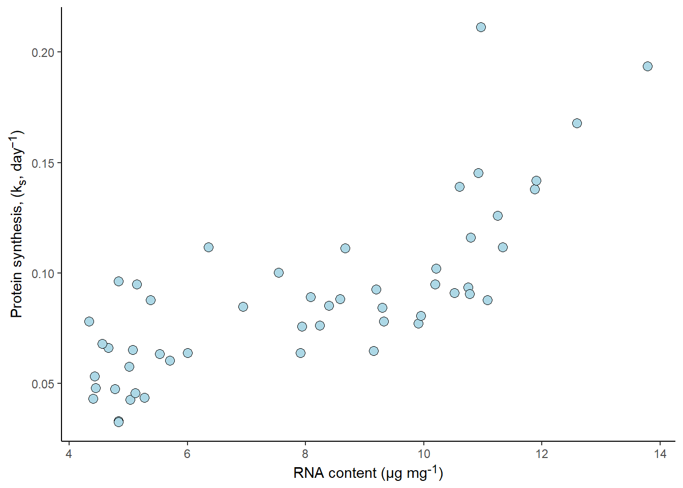
As with all code chunks, echo, warning, message etc. controls the output behaviour of the code chunk in the report. See the quarto documentation for more figure options
5.7 Saving figures as stand alone files
It is sometimes useful, and necessary to save figures in a stand alone file and not as part of a report, book or website. When creating a ggplot figure, the ggsave function is convenient for this purpose.
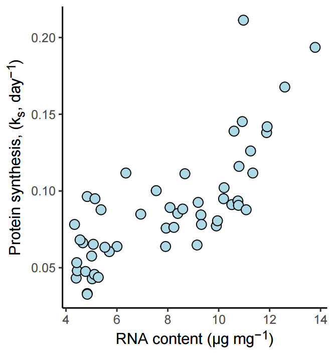
The ggsave function needs a filename for where to store the output figure, a plot as its input and options related to the size and type of output. Defining output formats makes it easy to get save a figure in a size suitable for your needs. For example, a scientific journal might accept figures for publication with a width of a whole printed page (17 cm), or half a page (8.5 cm). Let’s say that we aim for half a page with a slightly larger height than width. We will use this information when saving figures that we prepare.
p1 <- ggplot(data = millward, aes(RNA, protein_synthesis)) +
geom_point(size = 3, shape = 21,
fill = "lightblue") +
theme_classic() +
labs(
y = "Protein synthesis, (k<sub>s</sub>, day<sup>−1</sup>)",
x = "RNA content (μg mg<sup>-1</sup>)") +
theme(axis.title.y = element_markdown(),
axis.title.x = element_markdown(),
legend.title = element_markdown())
ggsave("figure1.pdf", p1, path = "figures", width = 8.5, height = 9,
units = "cm")The resulting figure is affected by the transformation to the output format, this means that we should expect a slightly different result based on the format we choose.
See the full ggsave documentation for more options.
5.8 Conclusions and further resources
ggplot2 gives us large flexibility to create simple to complex figures based on data. The ggplot2 package is popular because it is well documented and is designed to balance the complexity that comes with large flexibility using a concise syntax. Because of the many possibilities offered we have just scratched the surface of what is possible to do with the ggplot2 package. There are several good resources aimed at ggplot2 for going further: