# An example function
my_fun  <- function(arg1, arg2) { # Name and arguments of the function

        # This is the body
        sum <- arg1 + arg2

        return(sum)

}

my_fun(2, 4)Writing R functions and calculate a lactate threshold
For a comprehensive overview of writing functions in R, Chapter 19 in (Wickham and Grolemund 2017) contains an excellent introduction.
Why write functions
- You should invest in writing functions, if you plan to re-use code by copy paste more than once (Wickham and Grolemund 2017).
- Functions can make your code more readable, reusable and make sure you minimize errors.
- The DRY principle applies → Do not repeat yourself (Wickham and Grolemund 2017).
What is a function?
- R is easily “extended” through the creation of function.
- Functions can live inside package that you or someone else has written.
- Functions can also live in your environment after being defined in your script.
mean(),sd()mutate()andggplot()are examples of functions that comes with the basic installation of R or packages.- For a function to live in your environment, it must have a name
- The function can come with a set of arguments
- The actual mechanics of the function is defined in the body
Naming the function
- The same rules apply to naming functions as other R objects.
- (Wickham and Grolemund 2017) recommend longer and informative/descriptive names written in “snake_case” (as opposed to “camelCase”).
- Be consistent!
- Do not use names of other function!
Arguments
- A function may be defined with named arguments, this is the “input” of the function.
- An argument may be a data frame, a single value or vector that the function will use.
- The function can be used with the arguments used in their place or named out of place.
# An example function
my_fun  <- function(value1, value2) { # Name and arguments of the function

        # This is the body
        diff <- value1 - value2

        return(diff)

}

# these are different
my_fun(value2 = 1, value1 = 4)

my_fun(1, 4)
Body
- The function body defines the output of the function
- It usually makes use of the data/values/variables defined in the arguments and returns a given output
- Output can be any R object.
- The
return()function is used to explicitly make some part of the body to the output of the function
# An example function
my_fun  <- function(value1, value2) { # Name and arguments of the function

        # This is the body
        diff <- value1 - value2

        sum <- value1 + value2

        results <- list()

        results$diff <- diff
        results$sum <- sum

        return(results)

}

# these are different
my_fun(value2 = 1, value1 = 4)

my_fun(1, 4)
Environment
- If a variable is not defined in the function, R will try to look for it in the environment.
- It is considered good practice to not rely on variables not defined in the function
# An example function

# A variable defined outside the function
value1 <- 3


my_fun  <- function(value2) { # Name and arguments of the function

        # This is the body
        diff <- value1 - value2

        sum <- value1 + value2

        results <- list()

        results$diff <- diff
        results$sum <- sum

        return(results)

}

my_fun(value2 = 1)

my_fun(5)
Conditions, errors and messages
- Functions can include conditional sections, using
ifmakes it possible to make the function flexible depending on input variables
my_fun <- function(value1, value2, calculate.sum = FALSE) {

        if (calculate.sum == TRUE) {

                sum <- value1 + value2

                return(sum)

        } else {

                print("No sum calculated")

        }

}

# Calculates the sum
my_fun(2, 4, TRUE)

# Does not calculate the sum
my_fun(2, 4, FALSE)- A function can stop if the input variable is of the wrong type,
my_fun <- function(value1, value2) {

        if (!any(is.numeric(c(value1, value2)))) {

                stop("One or more values are not numeric")

        } else {

                sum <- value1 + value2

                return(sum)

        }

}

# Calculates the sum
my_fun(value1 = "error?", value2 = 4)

# Does not calculate the sum
my_fun(value1 = 2, value2 = 4)- There are several additional ways to create conditional operations (see (Wickham and Grolemund 2017)).
Group work
- Write a function that is reusable using this code:
z <- df$var1 - mean(df$var1, na.rm = TRUE) / sd(df$var1, na.rm = TRUE)Write a function that stops if the input is not a character vector
Write a function that calculates the standard deviation
\[s=\sqrt{\frac{\sum(x_i-\bar{x})^2}{n-1}}\]
# An example vector
x <- c(2, 5, 7, 8)

# Sum of squares
ss <- sum((x - mean(x))^2)

## Calculates standard deviation
s <- sqrt(ss / (length(x)-1))
A function to calculate lactate thresholds
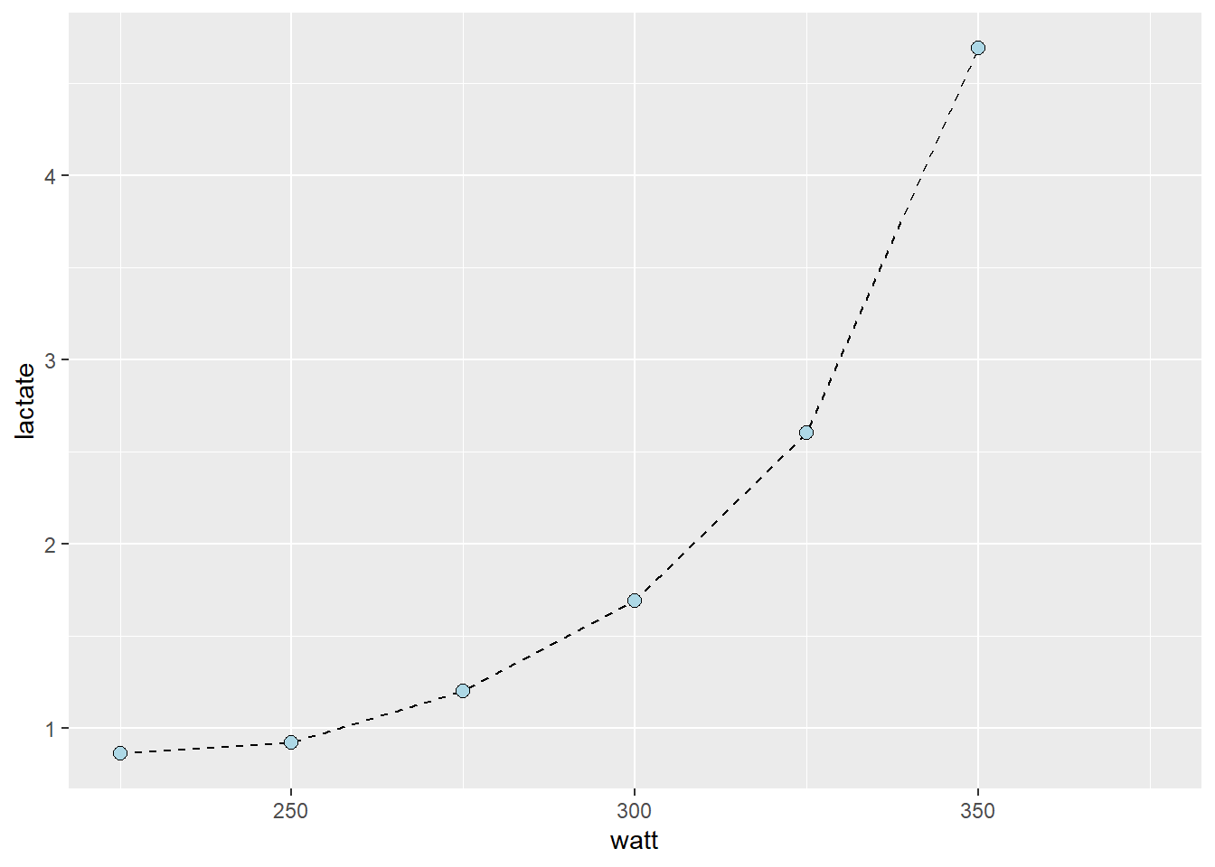
- Lactate threshold (LT) tests are commonly performed in the laboratory
- Calculations of the LT differs between labs and there are many methods
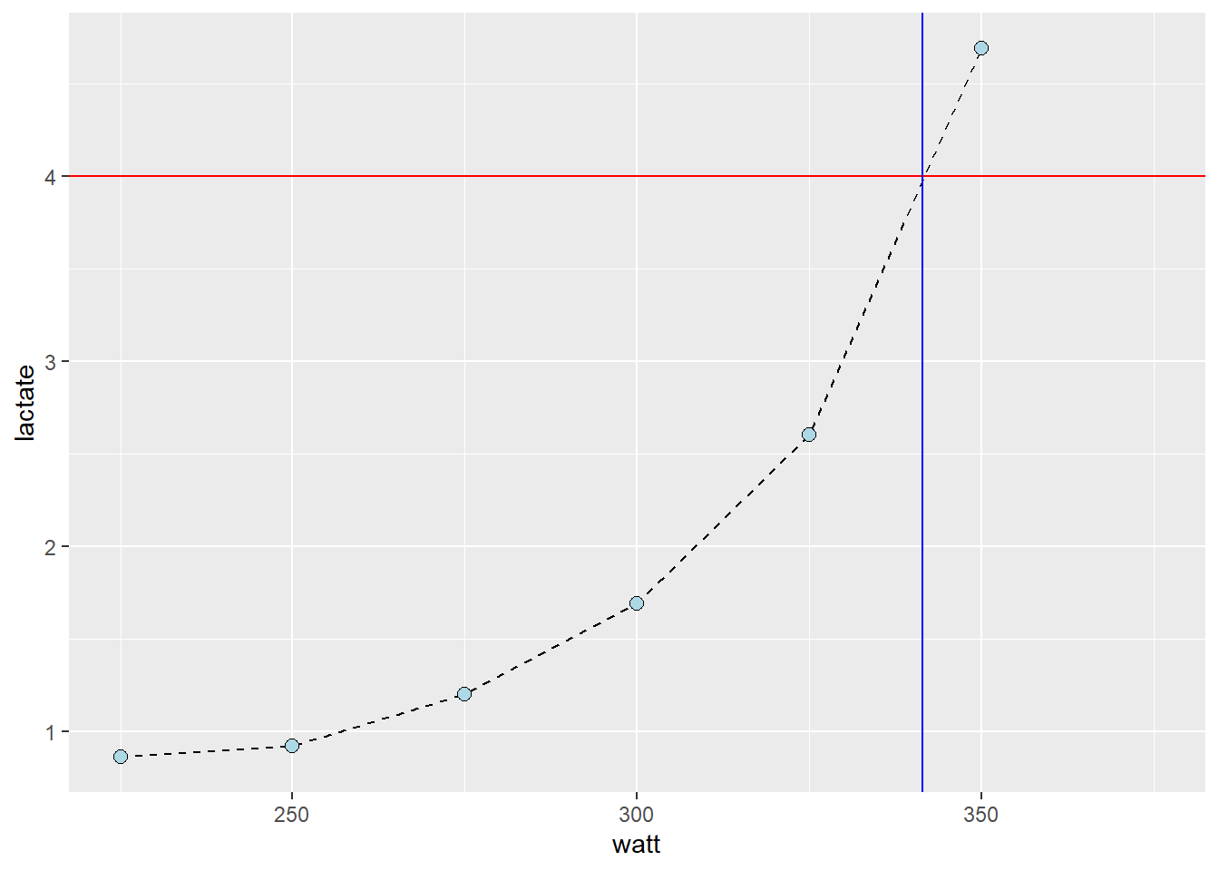
- A possible method is to calculate the power at a fixed lactate value (e.g. 4 mmoL L-1)
library(tidyverse)
library(exscidata)

data("cyclingstudy")


cyclingstudy %>%
  # Select columns needed for analysis
  select(subject, group, timepoint, lac.225:lac.375) %>%
  # Only one participant and time-point
  filter(timepoint == "pre", subject == 10) %>%
  # Pivot to long format data using the lactate columns
  pivot_longer(names_to = "watt",
               values_to = "lactate",
               names_prefix = "lac.",
               names_transform = list(watt = as.numeric),
               cols = lac.225:lac.375) %>%
  # Plot the data, group = subject needed to connect the points
  ggplot(aes(watt, lactate, group = subject))  +
  geom_line(lty = 2) +
geom_point(shape = 21, fill = "lightblue", size = 2.5) 
- Manually, we could estimate the watt at a specific lactate using ocular inspection
cyclingstudy %>%
  # Select columns needed for analysis
  select(subject, group, timepoint, lac.225:lac.375) %>%
  # Only one participant and time-point
  filter(timepoint == "pre", subject == 10) %>%
  # Pivot to long format data using the lactate columns
  pivot_longer(names_to = "watt",
               values_to = "lactate",
               names_prefix = "lac.",
               names_transform = list(watt = as.numeric),
               cols = lac.225:lac.375) %>%
  # Plot the data, group = subject needed to connect the points
  ggplot(aes(watt, lactate, group = subject))  +
  geom_line(lty = 2) +
  geom_point(shape = 21, fill = "lightblue", size = 2.5) +
  # Adding straight lines at specific values
  geom_hline(yintercept = 4, color = "red") +
  geom_vline(xintercept = 341.5, color = "blue")
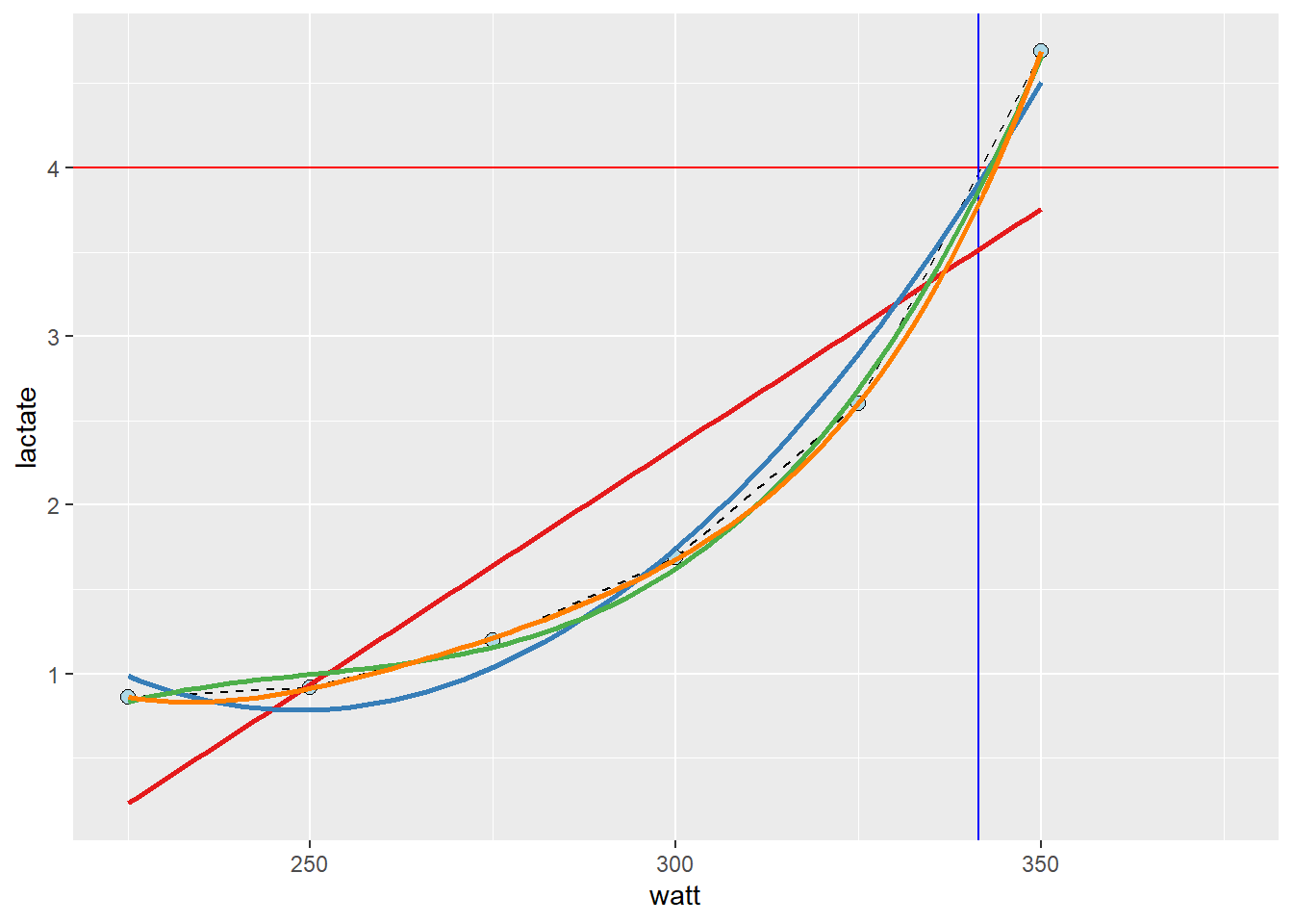
- A better approximation can be derived from the curve linear model
cyclingstudy %>%
  # Select columns needed for analysis
  select(subject, group, timepoint, lac.225:lac.375) %>%
  # Only one participant and time-point
  filter(timepoint == "pre", subject == 10) %>%
  # Pivot to long format data using the lactate columns
  pivot_longer(names_to = "watt",
               values_to = "lactate",
               names_prefix = "lac.",
               names_transform = list(watt = as.numeric),
               cols = lac.225:lac.375) %>%
  # Plot the data, group = subject needed to connect the points
  ggplot(aes(watt, lactate, group = subject))  +
  geom_line(lty = 2) +
  geom_point(shape = 21, fill = "lightblue", size = 2.5) +
  geom_hline(yintercept = 4, color = "red") +
  geom_vline(xintercept = 341.5, color = "blue") +
  # Adding a straight line from a linear model
  geom_smooth(method = "lm", se = FALSE, formula = y ~ x, color = "#e41a1c") +

  # Adding a polynomial linear model to the plot

  # poly(x, 2) add a second degree polynomial model.
  geom_smooth(method = "lm", se = FALSE, formula = y ~ poly(x, 2), color = "#377eb8") +
  # poly(x, 3) add a third degree polynomial model.
  geom_smooth(method = "lm", se = FALSE, formula = y ~ poly(x, 3), color = "#4daf4a") +
  # poly(x, 4) add a forth degree polynomial model.
geom_smooth(method = "lm", se = FALSE, formula = y ~ poly(x, 4), color = "#ff7f00") 
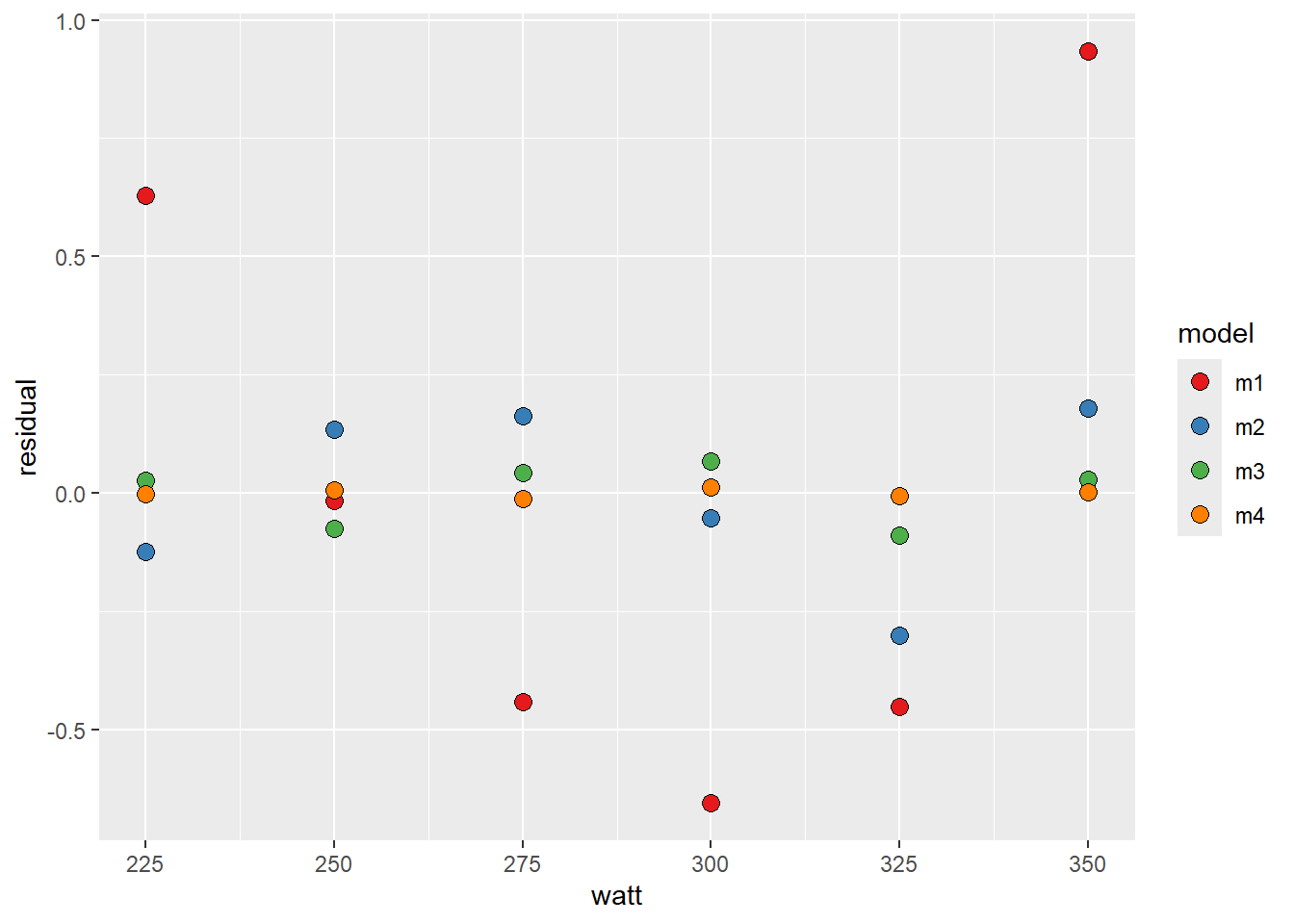
- These models are all “wrong but some are useful”1
lactate <- cyclingstudy %>%
  # Select columns needed for analysis
  select(subject, group, timepoint, lac.225:lac.375) %>%
  # Only one participant and time-point
  filter(timepoint == "pre", subject == 10) %>%
  # Pivot to long format data using the lactate columns
  pivot_longer(names_to = "watt",
               values_to = "lactate",
               names_prefix = "lac.",
               names_transform = list(watt = as.numeric),
               cols = lac.225:lac.375) %>%
  # Remove NA (missing) values to avoid warning/error messages.
  filter(!is.na(lactate))

# fit "straight line" model
m1 <- lm(lactate ~ watt, data = lactate)

# fit second degree polynomial
m2 <- lm(lactate ~ poly(watt, 2, raw = TRUE), data = lactate)

# fit third degree polynomial
m3 <- lm(lactate ~ poly(watt, 3, raw = TRUE), data = lactate)

# fit forth degree polynomial
m4 <- lm(lactate ~ poly(watt, 4, raw = TRUE), data = lactate)

# Store all residuals as new variables
lactate$resid.m1 <- resid(m1)
lactate$resid.m2 <- resid(m2)
lactate$resid.m3 <- resid(m3)
lactate$resid.m4 <- resid(m4)

lactate %>%
  # gather all the data from the models
  pivot_longer(names_to = "model",
               values_to = "residual",
               names_prefix = "resid.",
               names_transform = list(residual = as.numeric),
               cols = resid.m1:resid.m4) %>%
  # Plot values with the observed watt on x axis and residual values at the y
  ggplot(aes(watt, residual, fill = model)) + geom_point(shape = 21, size = 3) +

  # To set the same colors/fills as above we use scale fill manual
  scale_fill_manual(values = c("#e41a1c", "#377eb8", "#4daf4a", "#ff7f00"))
- Using the
predict()function we can predict lactate values at a specific power output. - We are modelling the effect of watt on lactate, so we are unable to input a specific lactate value, instead we could approximate with “inverse prediction
ndf <- data.frame(watt = seq(from = 225, to = 350, by = 0.1)) # high resolution, we can find the nearest10:th a watt

ndf$predictions <- predict(m3, newdata = ndf)

# Which value of the predictions comes closest to our value of 4 mmol L-1?
# abs finds the absolute value, makes all values positive,
# predictions - 4 givs an exact prediction of 4 mmol the value zero
# filter the row which has the prediction - 4 equal to the minimal absolut difference between prediction and 4 mmol
lactate_threshold <- ndf %>%
  filter(abs(predictions - 4) == min(abs(predictions - 4)))
Group work
- Write a function that calculates the lactate threshold using a fixed lactate value.
- The function should have arguments that defines the data and lactate value
- The output should be a value of the approximate watt at the fixed lactate
References
Wickham, Hadley, and Garrett Grolemund. 2017. R for Data Science: Import, Tidy, Transform, Visualize, and Model Data. 1st ed. Paperback; O’Reilly Media. http://r4ds.had.co.nz/.
Footnotes
See https://en.wikipedia.org/wiki/All_models_are_wrong↩︎