Statistical Power and Significance testing

Null hypothesis significance testing (NHST)

1. Choose a null-hypothesis, e.g. there is no differences between groups \(H_0:\mu_1 = \mu_2\), and a alternative hypothesis e.g. \(H_1:\mu_1 - \mu_2 \neq 0\)
2. Specify a significance level, usually 5% (or \(\alpha=0.05\)).
3. Perform an appropriate test, in the case of differences between means, a t-test and calculate the \(p\)-value
4. If the \(p\)-value is less than the stated \(\alpha\)-level we declare the result as statistically significant and reject \(H_0\).

• NHST is probably the most common way of making decisions about effects within quantitative sciences:

• NHST can be used to assess if e.g. groups are different or regression parameters are different than zero.

• NHST can be performed using the following steps:

NHST is a special flavour of hypothesis testing

• Two competing views on hypothesis testing were originally presented by Ronald A. Fisher on the one hand and Jerzy Neyman and Egon Pearson on the other hand.

NHST is a special flavour of hypothesis testing

Fisher	Neyman-Pearson
1. State \(H_0\)	1. State \(H_0\) and \(H_1\)
2. Specify test statistic	2. Specify \(\alpha\) (e.g. 5%) and \(\beta\)
3. Collect data, calculate test statistic and \(p\)-value	3. Specify test statistics and critical value
4. Reject \(H_0\) if \(p\) is small	4. Collect data, calculate test statistic, determine \(p\)
	5. Reject \(H_0\) in favour of \(H_1\) if \(p < \alpha\)

(Kline 2013)

Statistical power! If there is an effect, I will find it!

Statistical power (\(1-\beta\))!

• Neyman and Pearson extended Fishers hypothesis testing procedure with the concept of power.
• An alternative hypothesis can be stated for a specific value of e.g. a difference \(H_1: \mu_1-\mu_2 = 5\)
• Using this alternative hypothesis we can calculate the statistical power: The rate of rejecting \(H_0\) if the alternative hypothesis is true.
• The rate at which we fail to reject \(H_0\) if \(H_1\) is true is the Type 2 error rate (\(\beta\)).
• Statistical power is therefore: \(1-\beta\).

Errors in NHST

• There are two scenarios where we make mistakes, by rejecting \(H_0\) when it is actually true and not rejecting \(H_0\) when it is false.

	State of the world
Decision	\(H_0\) true	\(H_0\) false
Accept \(H_0\)		Type II error
Reject \(H_0\)	Type I error

Error rates in NHST

• We usually specify the level of Type I errors to 5%
• Another convention is to specify the power to 80%, this means that the risk of failing to reject \(H_0\) when \(H_0\) is false is 20%.
• These levels are chosen by tradition(!), but a well designed study is planned using well thought through Type I and II error rates.
• In the case of \(\alpha = 0.05\) and \(\beta=0.2\), Cohen (2013) pointed out that this can be thought of as Type I errors being a mistake four times more serious than Type II errors. (\(\frac{0.20}{0.05} = 4\))
• Rates could be adjusted to represent the relative seriousness of respective errors.

The \(p\)-value (again!)

• The \(p\)-value is the probability of obtaining a value of a test statistic (t) as extreme as the one obtained or more extreme under the condition that the null-hypothesis is true (sometimes written as \(p(t|H_0)\))

• We assume that the null is true and we calculate how often a result such as the one obtained, or even more extreme, would occur as a result of chance.

• The \(\alpha\)-level is the Type I error rate, the probability of rejecting \(H_0\) when it is actually true.

• Using \(\alpha = 0.05\) we simply declare significant when \(p<0.05\) (and accept that we will be wrong in 5% of an infinite number of studies), this is the Neyman-Person approach,

Interpreting \(p\)-values

• There are (commonly in scientific practice) two distinct ways of looking at the \(p\)-value, one where the \(p\)-value is a pre-specified threshold for decision (Neyman-Pearson), and one where the \(p\)-value is thought of as a measure of strength of evidence against the null-hypothesis (Fisher).

Interpreting \(p\)-values

• It is common practice to combine the two approaches in analysis of scientific experiments. Examples:

  • “There was not a significant difference between groups but the p-values suggested a trend towards …”
  • “The difference between group A and B was significant, but the difference between A and C was highly significant”

• According to the original frameworks, the mix (Fisher combined with Neyman-Pearson) may lead to abuse of NHST

Interpreting \(p\)-values

• Neyman and Pearson thought about \(\alpha\) and \(\beta\) as probabilities attached to the testing procedure.
• \(\alpha\) and \(\beta\) should be decided before the experiment and guide the researcher in making decisions.
• Controlling \(\alpha\) and \(\beta\) is about controlling error rates!
• Fisher believed that the \(p\)-value could serve as a statement about null-hypothesis given the sample…

(Dienes 2008)

The \(\alpha\)-error and statistical power are related

This means that there is always a trade-off between power an type-I errors! Unless you can have large n!

What does a power of 0.5 mean?

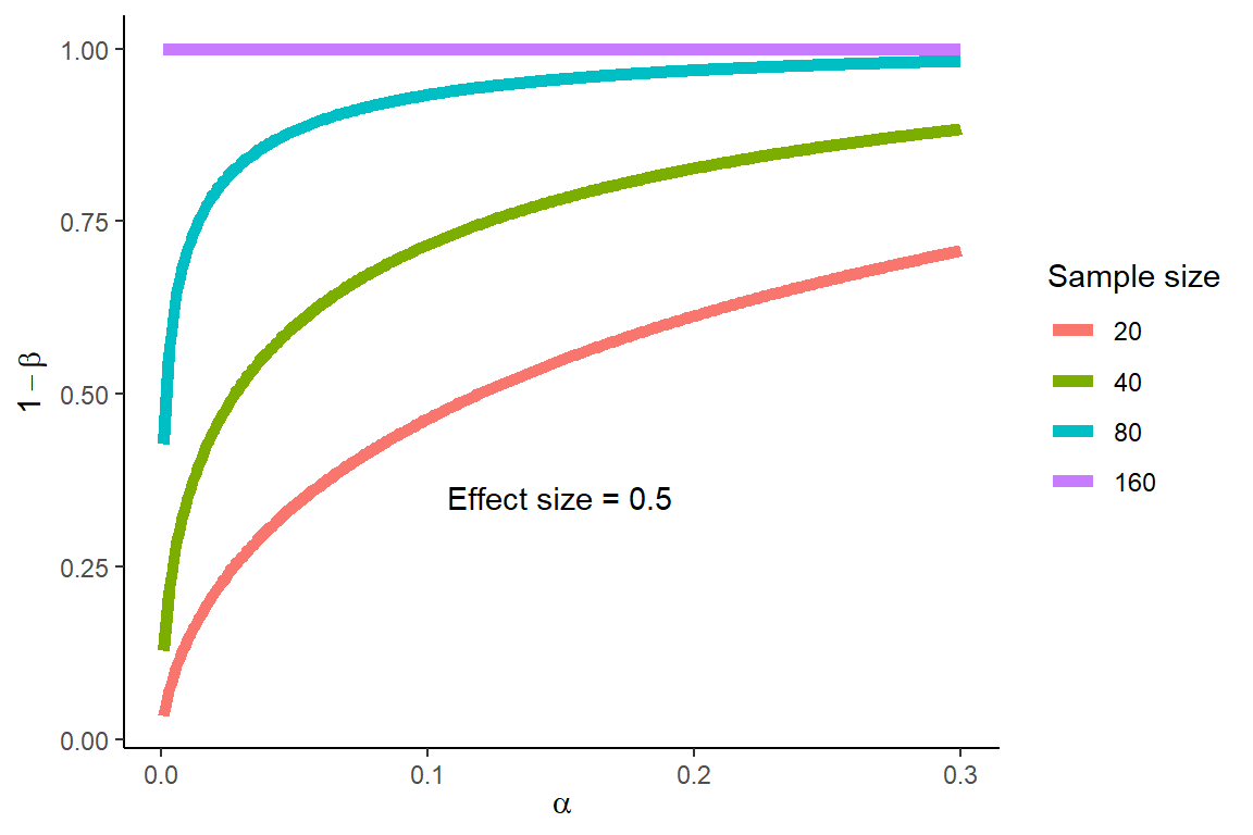
Error rates in NHST, an example

• If a study tries to determine if a novel treatment with no known side-effects should be implemented, failure to detect a difference compared to placebo when there is a difference (Type II error) would be more serious than to detect a difference that is not true (Type I error).

• In this case error rates could be adjusted to reflect this, decrease possibility Type II errors by increasing the possibility of Type I errors.

Power analysis in NHST

• This is a question of cost as more participants means more work
• It is a question of ethics as more participants means that more people are subjected to risk/discomfort.
• We aim to recruit as many participants as is necessary to answer our question.
• We state our \(H_0\) and \(H_1\) (according to the Neyman-Pearson tradition).
• When we have specified \(H_1\) we can perform power analysis and sample size estimation.

• The \(H_1\) has a special function, this can be seen as the smallest meaningful difference between conditions under study, the difference we want to be able to detect.

Power analysis, an example

• A 1 kg difference in lean mass increases is considered a meaningful difference after 12 weeks of training.
• The standard deviation from previous studies is used to estimate the expected variation in responses to 12 weeks of resistance training (\(\sigma = 2.5\)).
  
• To calculate the required sample size we first must calculate a standardized effect size, also known as Cohen’s \(d\).
• We can standardize our “effect size” of 1 kg by dividing by the SD \(d = \frac{1}{2.5}= 0.4\)

• We want to compare the muscle mass gains as a result of two resistance training protocols.

Effect sizes

• The effect size is the primary aim of an experiment, we wish to know the difference, correlation, regression coefficient, percentage change…
• The effect size can be standardized (e.g. divided by the standard deviation or calculated as e.g. a correlation).

Power analysis, an example cont.

• Let’s say that the Type I error is four times more serious than the Type II error, and that we would accept to be wrong in rejecting \(H_0\) at a rate of 5%.

\[\alpha=0.05,~\beta=0.2,~d = 0.4\]

• Given these specifics we would require 100 in each group to be able to show a meaningful difference with the power set to 80%.

• We must specify \(\alpha\) and \(1-\beta\) to calculate the required sample size!

• This is a big study what if we examine the smallest difference we can detect using a set sample size

Mean difference between groups vs. number of participants per group

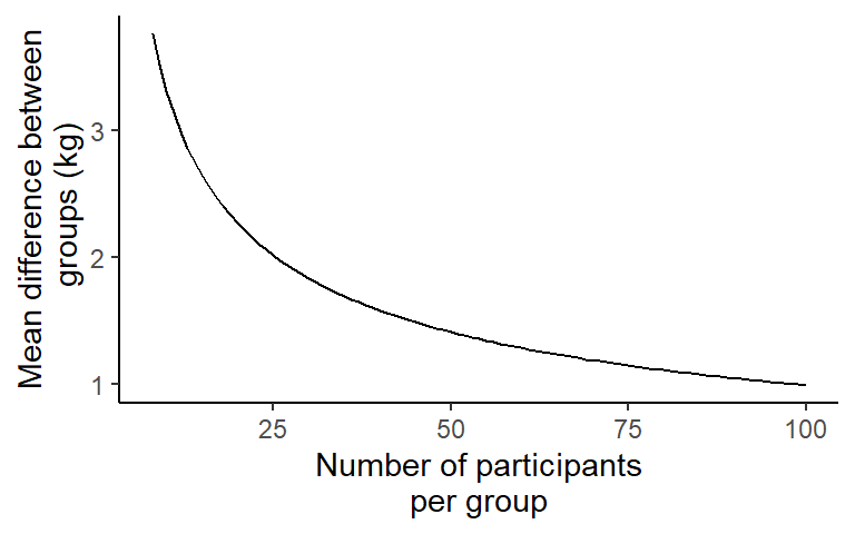
Power analysis

Statistical power is influenced by:

• The \(\alpha\) level
• The direction of the hypothesis (negative, positive or both ways different from \(H_0\))
• Experimental design (e.g. within- or between-participants)
• The statistical test
• Reliability of test scores

Critique of NHST

• NHST with \(p\)-values tend to create an “either-or” situation, gives no answer about the size of an effect
• Test statistics are related to sample size, small effects can be detected using big sample sizes
• Built in to the NHST framework is the acceptance of a proportion of tests being false positive (\(\alpha\)), the risk of getting false positives increases with the number of tests.

NHST and magnitude of an effect

• “The training group gained 3 kg in muscle mass from pre- to post-training (p<0.05)”

Some scientists wants to use the p-value as a signal of importance…

Statistical significance and clinical significance

Large sample sizes can make small effect sizes statistically significant. Example, (Lee 2010):

• Objective: To examine the association of different amounts of physical activity with long-term weight changes among women consuming a usual diet.

• Design: Prospective cohort study, following 34,079 healthy, US women (mean age, 54.2 years) from 1992–2007. At baseline, 36-, 72-, 96-, 120-, 144- and 156-months’ follow-up, women reported their physical activity and body weight.

Statistical significance and clinical significance

• Results: Women gained a mean of 2.6 kg throughout the study. In multivariate analysis, compared with women expending \(\geq\) 21 MET-hr/week, those expending 7.5-<21 and <7.5 MET-hr/week gained 0.11 kg (SD=0.04; P=0.003) and 0.12 kg (SD=0.04; P=0.002), respectively, over a mean interval of 3 years.

(Lee 2010)

Results

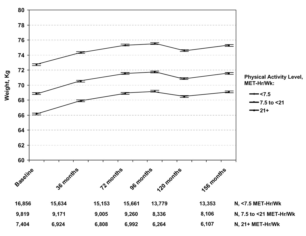
(Lee 2010)

Making the wrong decision 5% of the time

• Given that NHST accepts mistakes at a rate of \(\alpha\), every \(\frac{1}{\alpha}=20^{th}\) test result will be false!
• The Neyman-Pearson approach is to only do NHST with an pre-specified \(\alpha\)-level
• One must also avoid making up hypotheses after the test.
• If you do multiple tests, family-wise corrections can be made, e.g. the Bonferroni correction: \(\alpha_{Bonferroni}=\frac{\alpha}{n~tests}\)
• For statistical significance to be reached, the \(\alpha_{Bonferroni}\) threshold must be reached.

What can the corrected \(p\)-value account for?

• A statistical hypothesis test using the Neyman-Pearson approach is about error-control.
• A single test has specified errors, but these are affected by e.g. sequential testing, sneak-peaks on the data, issues with randomization and study designs…
• A large proportion of tests will not be “severe enough” to reject \(H_0\)
• We are not always aware of when we adjust \(\alpha\) the wrong way

(Mayo 2018; Dienes 2008)

This is a note on the error control and severe testing proposed by Mayo.

Sequential testing will lead to significant results… eventually

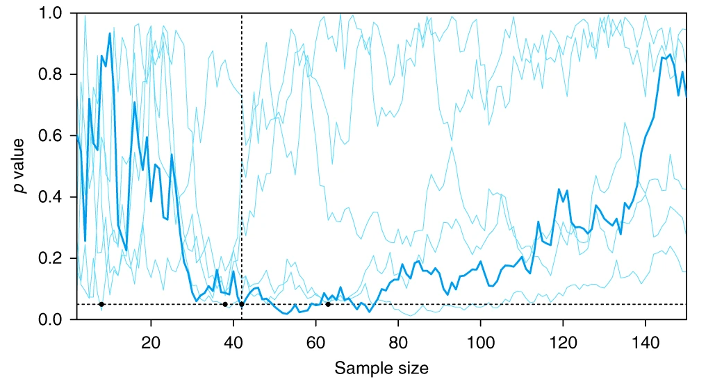
Albers (2019)

The philosophy of statistics, in practice, is a mix!

Journal of Physiology: For a given conclusion to be assessed, the exact p-values must be stated to three significant figures even when ‘no statistical significance’ is being reported. These should be stated in the main text, figures and their legends and tables. The only exception to this is if p is less than 0.0001, in which case ‘<’ is permitted. Trend statements are not permitted (i.e. ‘x increased, but was not significant’). Where there are many comparisons, a table of p values may be appropriate.

What does the p-value mean?

All groups regained weight after randomization by a mean of 5.5 kg in the self-directed, 5.2 kg in the interactive technology–based, and 4.0 kg in the personal-contact group… Those in the personal-contact group regained a mean of 1.2 kg less than those in the interactive technology–based group (95% CI, 2.1-0.3 kg; P=.008).

What does the p-value mean? Svetkey at al…

1. …have absolutely disproved the null hypothesis (that there is no difference between the population means).
2. … have found the probability of the null hypothesis being true.
3. … have absolutely proved their experimental hypothesis (that there is a difference between the population means).

Questions adopted from (Dienes 2008).

What does the p-value mean? Svetkey at al…

4. … can deduce the probability of the experimental hypothesis being true.
5. … know the probability that you are making the wrong decision, if you decided to reject the null hypothesis.
6. … have a reliable experimental finding in the sense that if, hypothetically, the experiment were repeated a great number of times, you would obtain a significant result on 95 % of occasions.

Questions adopted from (Dienes 2008).

A complement or alternative to NHST: Estimation

• Instead of testing against a null-hypothesis, estimation aims at finding a point estimate of the parameter of interest
• Secondly we want to find an interval estimate of the parameter
• This can be done using confidence intervals.
• Confidence intervals provides an point-estimate together with a range of plausible values of the population parameter.

Estimation, an example

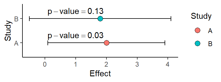
• What conclusions can be drawn from the two studies (using NHST vs. estimation)?

(Cumming 2012)

Estimation

• In addition to giving a interval representing the precision of the estimate, the confidence interval can be used to assess the clinical importance of a study.
• Are values inside the confidence interval large (or small) enough to care about in a clinical sense (e.g. weight gain study)

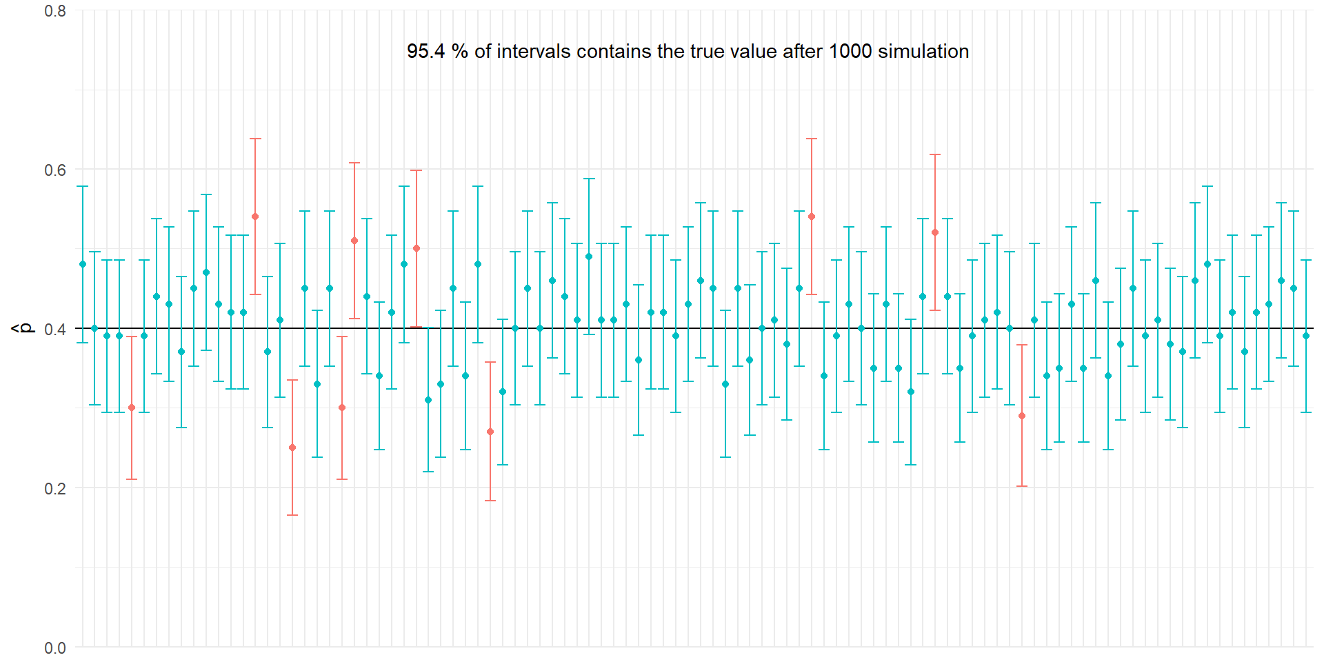
Estimation using confidence intervals still has the draw-back of NHST

Alternatives to Null-hypothesis testing

• If you are interested in quantifying the probability of obtaining the population parameter, given your prior understanding → Bayesian statistics!

• If you want to quantify the relative evidence in favour of a hypothesis over another based on your data → Likelihood inference!

References

Albers, Casper. 2019. “The Problem with Unadjusted Multiple and Sequential Statistical Testing.” Nature Communications 10 (1): 1921. https://doi.org/10.1038/s41467-019-09941-0.

Cohen, Jacob. 2013. Statistical Power Analysis for the Behavioral Sciences. 0th ed. Routledge. https://doi.org/10.4324/9780203771587.

Cumming, Geoff. 2012. Understanding the New Statistics : Effect Sizes, Confidence Intervals, and Meta-Analysis. Multivariate Applications Series. New York: Routledge.

Dienes, Zoltan. 2008. Understanding Psychology as a Science: An Introduction to Scientific and Statistical Inference. New York: Palgrave Macmillan.

Kline, Rex B. 2013. Beyond Significance Testing: Statistics Reform in the Behavioral Sciences, 2nd Ed. Beyond Significance Testing: Statistics Reform in the Behavioral Sciences, 2nd Ed. Washington, DC, US: American Psychological Association. https://doi.org/10.1037/14136-000.

Lee, I-Min. 2010. “Physical Activity and Weight Gain Prevention.” JAMA 303 (12): 1173. https://doi.org/10.1001/jama.2010.312.

Mayo, Deborah G. 2018. Statistical Inference as Severe Testing : How to Get Beyond the Statistics Wars. Cambridge ; New York, NY: Cambridge University Press.