Estimating a sampling distribution
Population and sample
- When we are interested in continuous data, the sample mean is unbiased estimate of the population parameter (the population mean).
The population mean:
\[\mu=\frac{\sum{X_i}}{N}\]
The sample mean:
\[\bar{x}=\frac{\sum{x_i}}{n}\]
Measures of dispersion
Central tendency is captured by the “center of gravity” in the data, however, we might also want to know something about its variation.
The population variance is the average (squared) difference from the mean
As the population parameters are unknown, we estimate them with our sample
\[\sigma^2 = \frac{\sum_{i=1}^{N}{(X_i-\mu)^2}}{N}\]
\[s^2 =\frac{\sum_{i=1}^{n}{(x_i-\bar{x})^2}}{n-1}\]
The sample variance
- The sample variance is an unbiased estimate of the population if we use \(n-1\) otherwise we will tend to underestimate the population values.
\[s^2 =\frac{\sum_{i=1}^{n}{(x_i-\bar{x})^2}}{n-1}\]
Variance and the standard deviation
- The variance is the average squared deviation from the mean
- The standard deviation (\(s\)) is the square root of the variance, thus on the same scale as the mean
\[s = \sqrt{\frac{\sum{(x_i-\bar{x})^2}}{n-1}}\]
Sampling distributions
- Any statistic can be calculated from a sample and used as an estimation of the population parameter.
- As an example, the sample mean (\(\bar{x}\)) is an unbiased estimator of the population mean, we can know this because the average of repeated samples from a population will be close to the population mean (\(\mu\)).
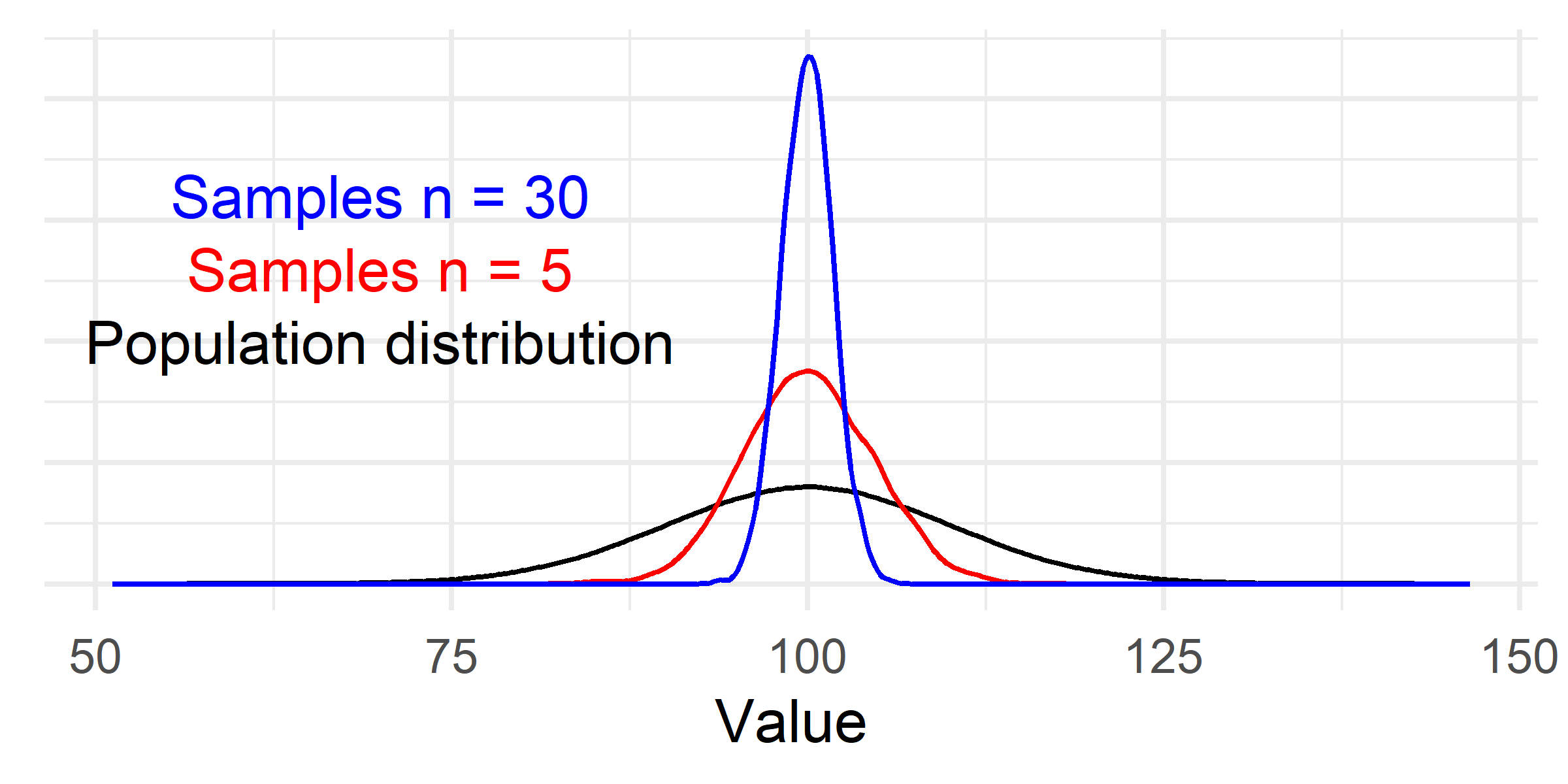
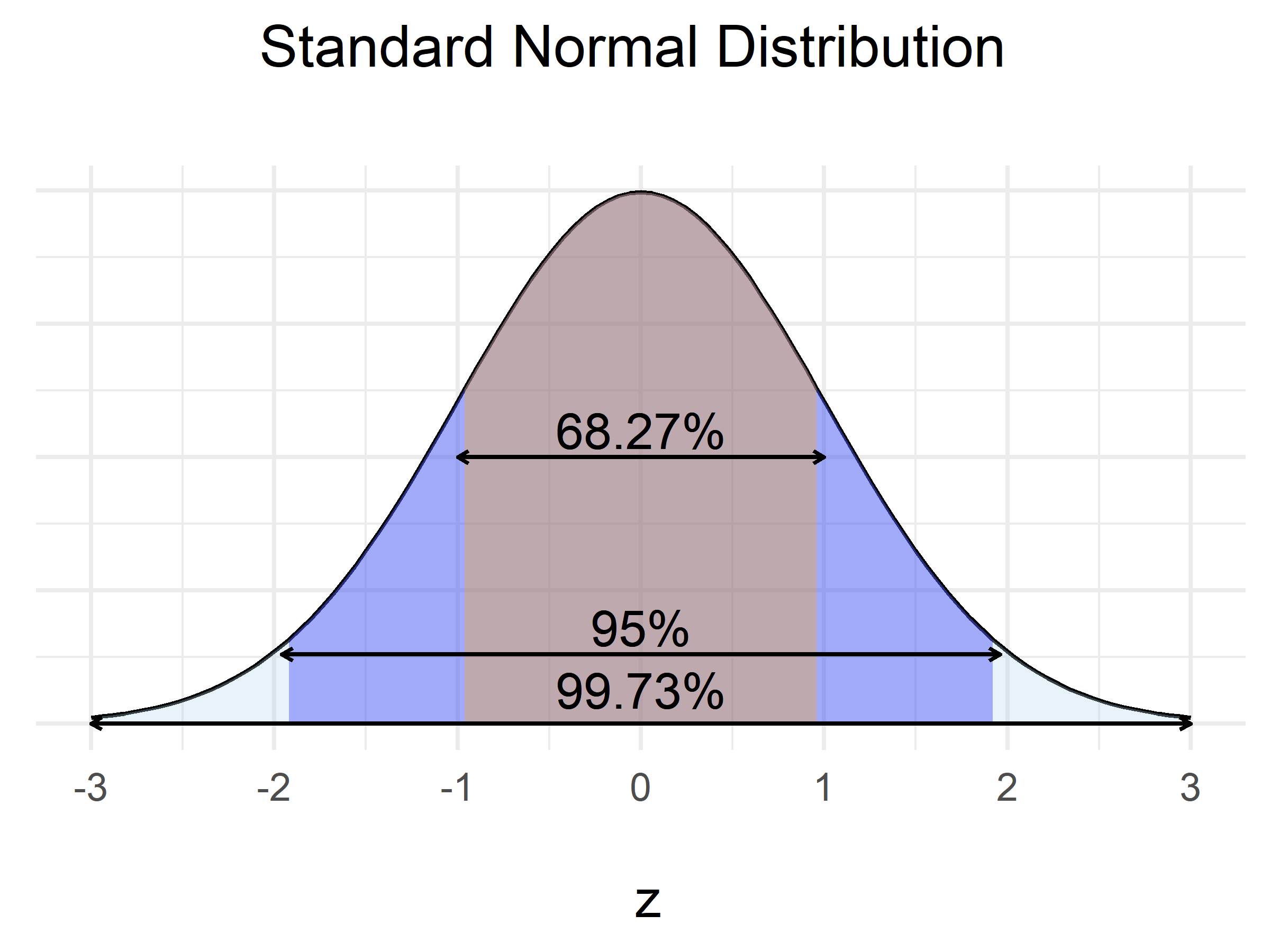
The distribution of samples will have a “normal” shape irrespective of the underlying population distribution!
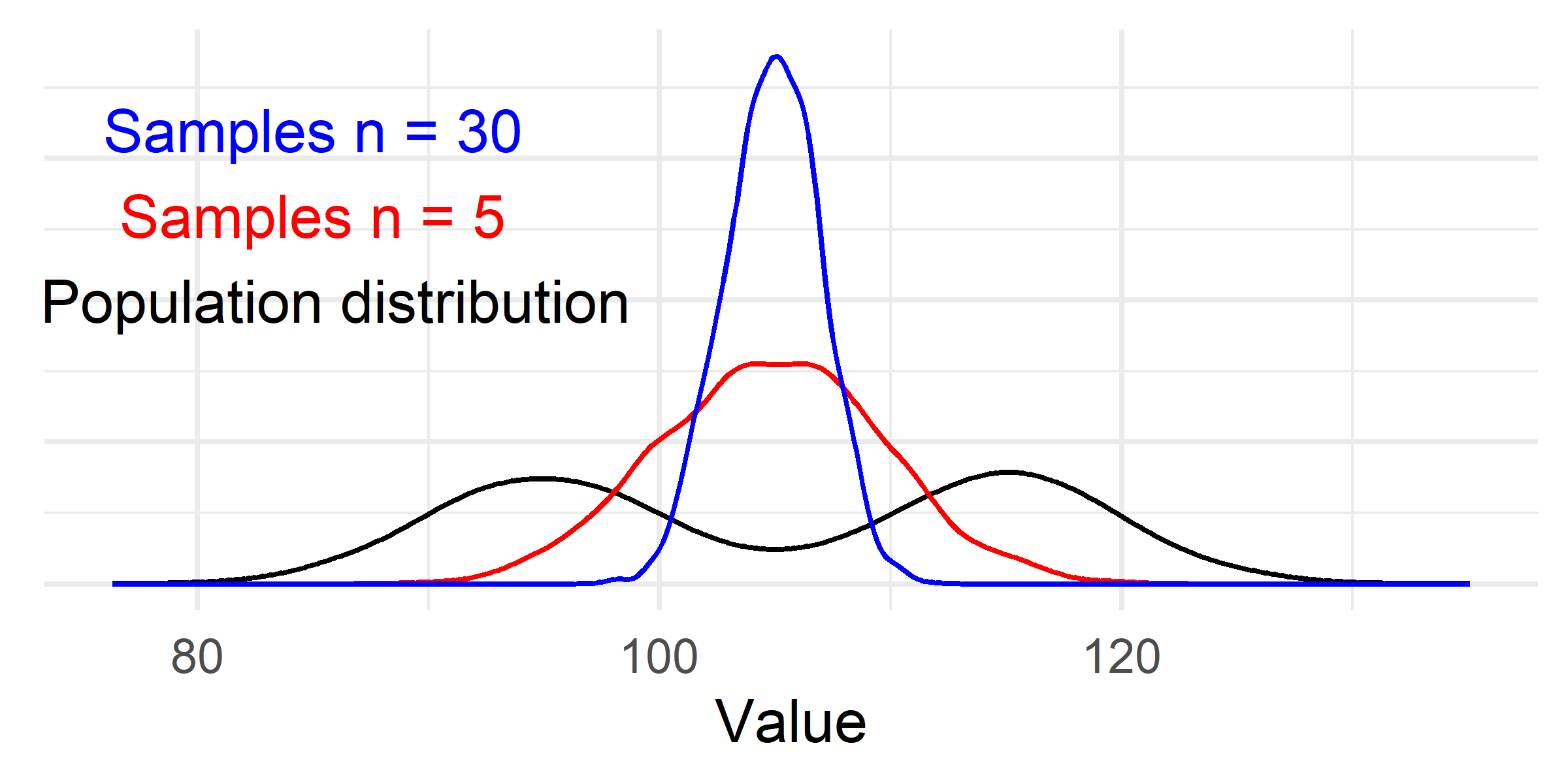
The distribution of samples will have a “normal” shape irrespective of the underlying population distribution!
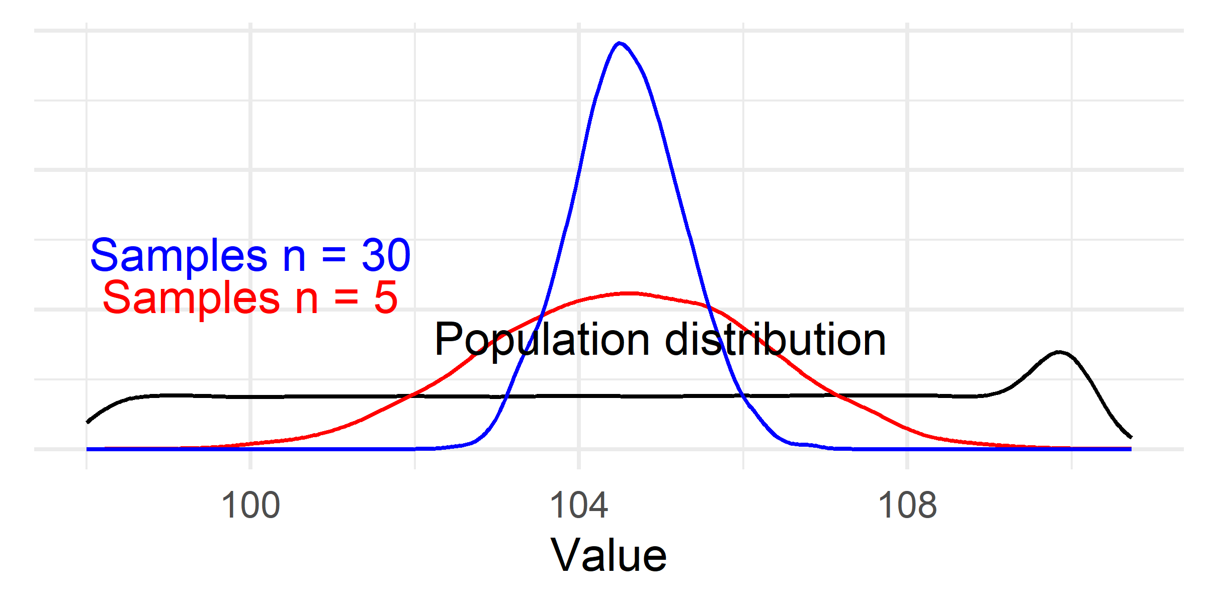
The Normal Distribution
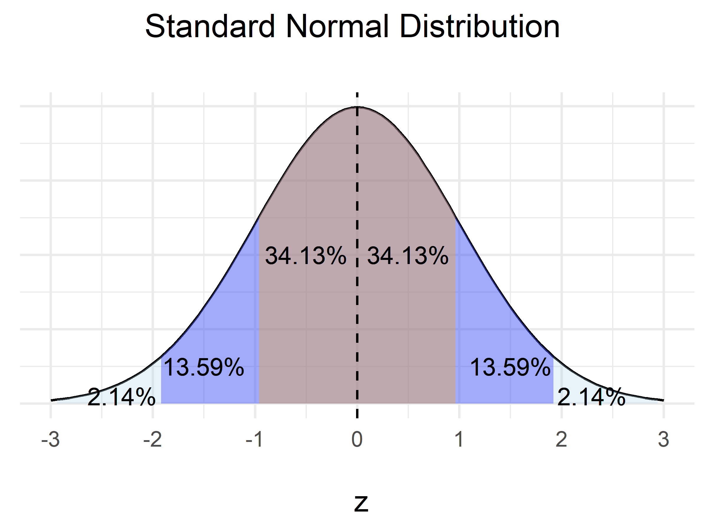
The Normal distribution
Sampling distributions
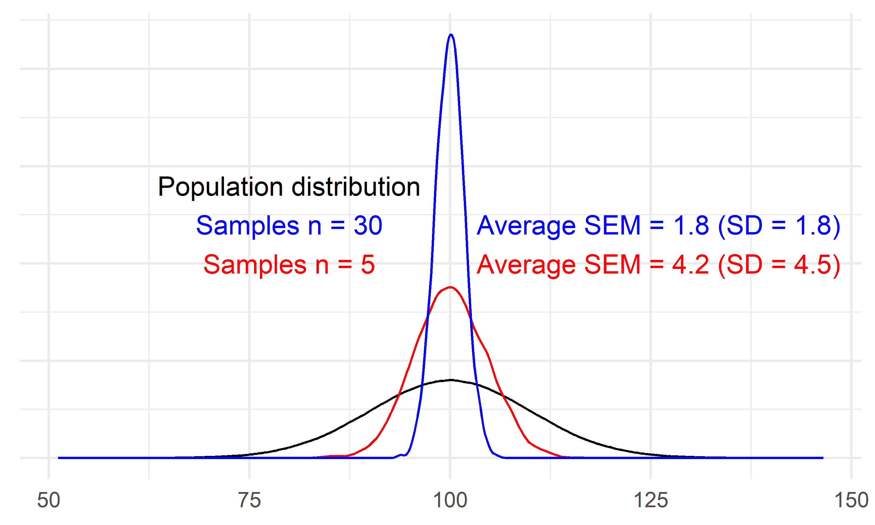
- The variation (standard deviation) of a distribution of averages is affected by the sample size.
- This variation can be estimated from samples and is known as the standard error.
- The sample standard error is an estimate of the standard deviation of the sampling distribution!
\[SE = \frac{s}{\sqrt{n}}\]
Sampling distributions
Hypothesis testing
Based on the estimate of the sampling distribution we can device a test, to test if a value exists within specified range.
95% of all values lies within \(\pm 1.96\times \sigma\) from the mean in a normal distribution, this leaves us with an uncertainty of 5%.
However, due to problems with proving a theory or hypothesis, we instead test against a null-hypothesis.
The null hypothesis \(H_0\) is constructed to contain scenarios not covered by the alternative hypothesis \(H_A\)
Hypothesis tests - a two sample scenario
The null hypothesis is that the mean of group 1 is similar to group 2 \(H_0: \mu_1 - \mu_2 = 0\)
To reject this hypothesis, we need to find support for \(\mu_1 - \mu_2 \neq 0\)
We want to do this with some specified error control, usually 5%. We accept that we will wrong in a specified number of cases.
We can calculate a 95% confidence interval of the difference
A 95% confidence interval for small samples
Upper bound: \[\bar{x} + t_{1-\alpha/2} \times SE\] Lower bound: \[\bar{x} - t_{1-\alpha/2} \times SE\]
- \(\bar{x}\) is the difference in means between groups.
- The standard error (\(SE\)) estimates the standard deviation of the sampling distribution
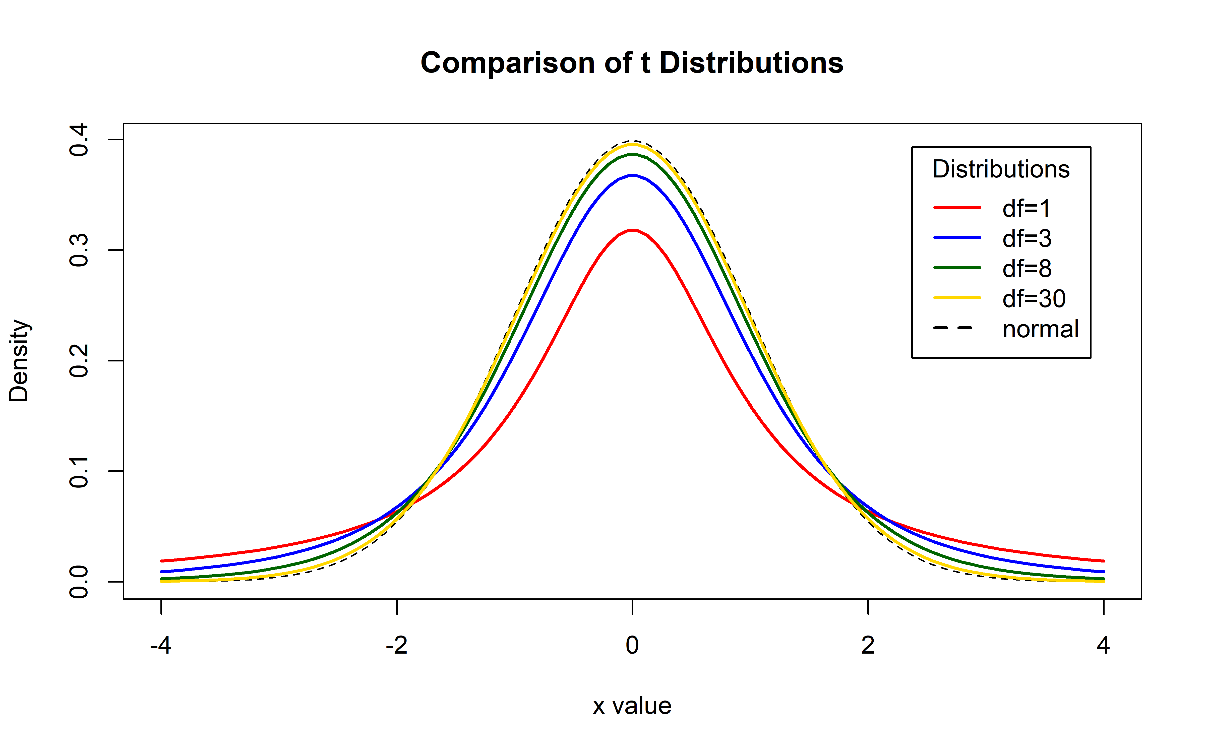
- \(t_{1-\alpha/2}\) represents the area under probability distribution curve containing 95% of all values.
- The \(t\)-distribution is used instead of the normal distribution since it can capture deviations from the Normal distribution due to the sample size.
The t-distribution
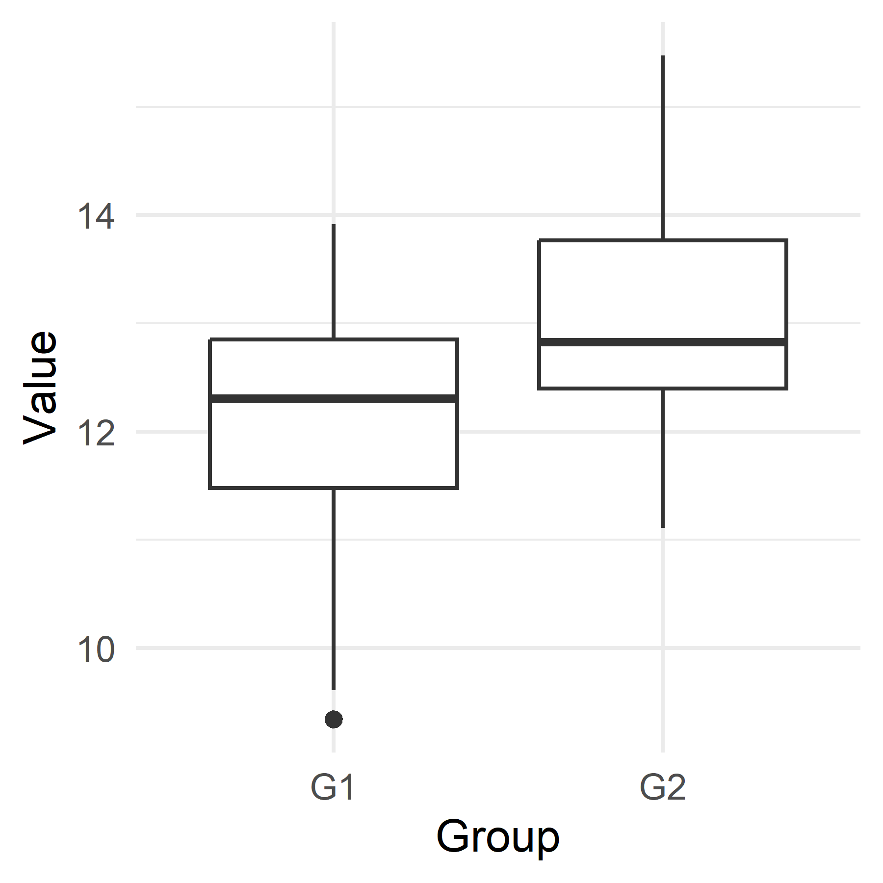
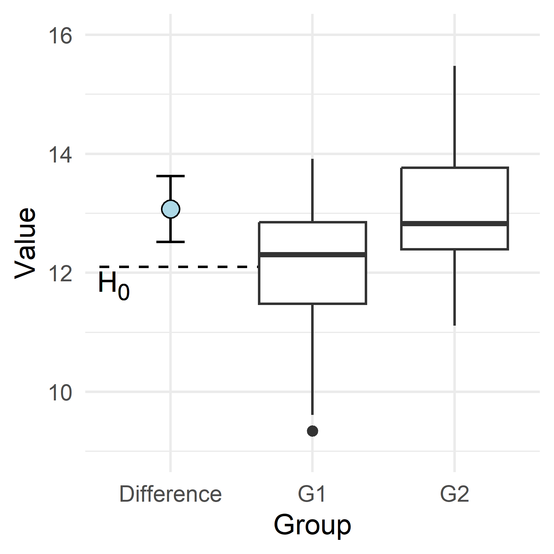
A case with samples from two groups
A 95% confidence of the difference in means
Two groups are compared, the \(H_0\) is that there is no difference between the groups: \(H_0: \mu_1 = \mu_2\)
The difference between the groups are estimated to \(\mu_2 - \mu_1 =\) 0.97
The 95% confidence interval is \(m_2 - m_1 \pm t_{\alpha/2} \times SE(m_2 - m_1)\) where the \(SE(m_2 - m_1)\) is the standard error of the difference.
A 95% confidence of the difference in means
Summary
- We can estimate population parameters using a random sample from the population
- The calculated sample standard error is an estimate of the standard deviation of a sampling distribution
- Using a probability density function like the \(t\)- or \(z\)-distribution, we can estimate a range a plausible values of a population parameter (e.g. mean).
- We can test if a estimated interval contains the null hypothesis, if not we can reject \(H_0\).