Writing reports in Quarto (or R markdown)
Basics: Quarto and Rmarkdown
- Quarto and R Markdown a special kind of scripts where text and computer code can be combined to generate reports.
- Under the hood, a report generator is converting code and plain text to an output format such as html, pdf or docx (more formats are available).
- Quarto is a new, well documented format that gives extra flexibility, but also requires installation of extra software.
- R Markdown is also, see e.g. R Markdown, R Markdown: The Definitive Guide
Code execution and the environment
- When a quarto or Rmarkdown file is “knitted” or compiled, the source file looks for additional files in the same directory as the source file is saved.
- Working in a RStudio projects makes it easy to work with the report interactively as you can use relative paths.
- RStudio has an excellent guide to its project feature
RStudio projects
- A projects is a collection of settings together with a root directory.
- This means that you will be able to work with relative paths.
- If reading a
csvfile using relative paths, your code will look like this from a project.
Absolute paths
- If your are using absolute paths, reaching the same operation could look like this
A basic structure for projects
RStudio projects helps you create good habits for reproducible analysis as all analyses are conducted within a stand-alone folder structure. Your data and scripts can be shared.
Use a basic structure for all projects:
My-project
        |
        |-.Rproj        (The project settings)
        |--/data        (Contains all data needed for your analysis)
        |--/R           (Contains all scripts/R-files)
        |--/output      (Collection of all output files)
Writing in Quarto/R Markdown
- The basic syntax in quarto/R Markdown files is markdown. Markdown makes it easy to format text without point-and-click as all formatting can be added with syntax, example:
This text is an example of the markdown syntax which includes **bold**, *italic*,
^super^ and ~subscript~ and ~~striketrough~~
Resulting in:
This text is an example of the markdown syntax which includes bold, italic, super and subscript and
striketrough
Markdown - More on text formatting (html)
We can also use html for <sub>subscripts</sub>
and <sup>superscript</sup>
We can also use html for subscripts and superscript
Markdown - More on text formatting (latex)
Mathematical formulas can be added inline with $y_i \sim \operatorname{Normal}(\mu_i, \sigma)$

or as a block, using

$$
y = \beta_0 + \beta_1 \times x_1 + \epsilon
$$
Mathematical formulas can be added inline with \(y_i \sim \operatorname{Normal}(\mu_i, \sigma)\)
or as a block, using
\[ y = \beta_0 + \beta_1 \times x_1 + \epsilon \]
Markdown lists
A list can be unordered and ordered

* Item A
    + Item x


1. Item 1
2. Item 2
    i) Item i
A list can be unordered and ordered
- Item A
- Item x
- Item 1
- Item 2
- Item i
Markdown tables
| Left |Center|Right|
| :--- |:---: |---:|
|Text | Text| Text|
|35| 3| 999|

: A table caption
| Left | Center | Right |
|---|---|---|
| Text | Text | Text |
| 35 | 3 | 999 |
Adding images

Cross-referencing
- With cross-referencing it is possible to reference images, tables, equations etc.
- A cross reference requires an identifier
{#fig-inn}
See [@fig-inn] for an example ...
See Figure 1 for an example …
Code chunk options
- Output from code chunks can be tables, figures or text used in the report.
- Code chunk options lets you specify, for example
- Figure captions, figure short-captions
- If code, messages or warnings should be shown
- Labels used for cross-referencing
- Caching (saving computations of a code block if unchanged)
Code chunk options syntax
#| echo: false
#| message: false
#| warning: false
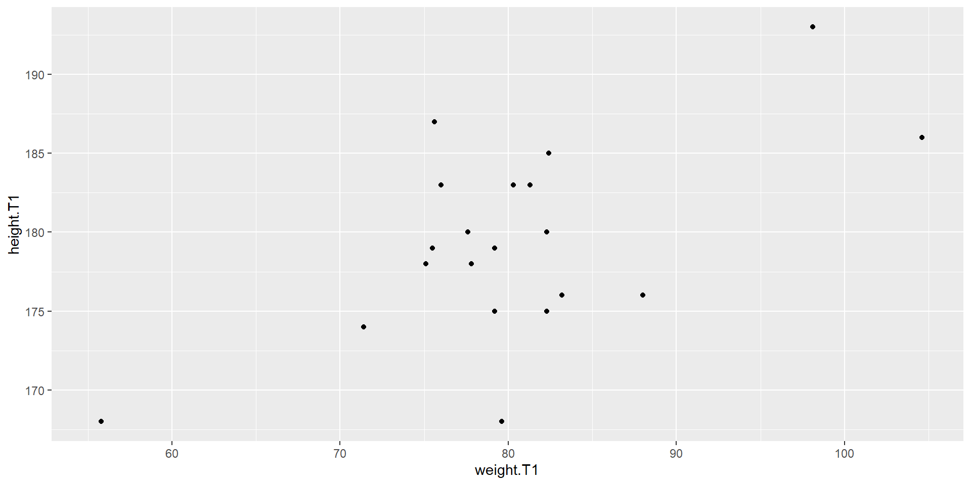
#| label: fig-example
#| fig-cap: "An example figure"


library(exscidata); library(tidyverse)

cyclingstudy %>%
        ggplot(aes(weight.T1, height.T1)) + geom_point()

Inline code
- Code may be included inline to include code generated outputs
- To include the variable in the text:
Bibliographies
- Bibliographies/Citations may be added to reports using a external bibliography file. A simple format is bibtex
- Pubmed entries can be searched using TexMed
- In the visual editor, bibliographies can be easily created
Where to find help?
- The quarto documentation is really good.
- A lot of examples on quarto is available trough google!
See the.